enter a function in cell D 36 based on the payment and Loan details from chapter 6 worksheet that calculates the amount of interest paid on the first payment be sure to use the appropriate absolute relative or mixed cell references fill out E36 and f36 with the appropriate formulas

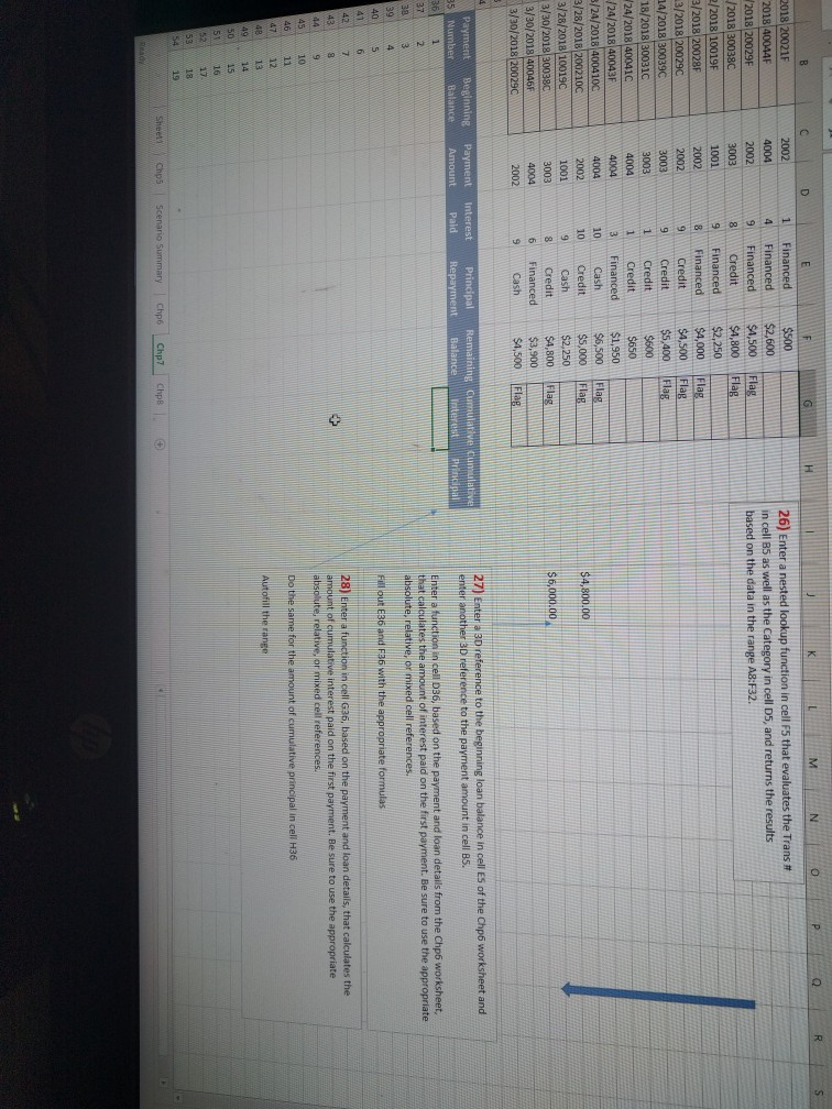
KLM 0 QRS Financed 1 4 $500 $2,600 $4,500 $4,800 $2,250 26) Enter a nested lookup function in cell FS that evaluates the Trans # in cell B5 as well as the Category in cell Ds, and returns the results based on the data in the range A8:F32. SA,000 $4,500 2018 20021F 2018 40044F 2018 20029 /2018 300380 2/2018 10019 3/2018 20028 3/2018 200290 74/2018 30039C 18/2018 300310 24/2018 400410 /24/2018 40043 B/24/2018 4004100 3/28/2018 2002100 3/28/2018 100190 3/30/2018 300380 3/30/2018 400467 3/30/2018/200290 2002 4004 2002 3003 1001 2002 2002 3003 3003 4004 4004 4004 2002 1001 3003 4004 2002 Financed Financed Credit Financed Financed Credit Credit Credit Credit Financed Cash Credit Cash Credit Financed Cash $5,400 $600 $650 $1,950 $6,500 $5,000 $2,250 $4,800 $3,900 $4,500 $4,800.00 $6,000.00 Beginnine Balance Payment Interest Amount Pald Principal Repayment Remain Balance 27) Enter 3D reference to the beginning loan balance in cell ES of the Chp6 worksheet and enter another 3D reference to the payment amount in cell B5. Payment 35 Number 361 372 1383 394 Enter a function in cell D36, based on the payment and loan details from the Chp worksheet, that calculates the amount of interest paid on the first payment. Be sure to use the appropriate absolute, relative, or mixed cell references. Fill out E36 and F36 with the appropriate formulas 28) Enter a function in cell G36, based on the payment and loan details, that calculates the amount of cumulative interest paid on the first payment. Be sure to use the appropriate absolute, relative, or mixed cell references. Do the same for the amount of cumulative principal in cell H36 BREGA TORNA Autofill the range Sweet hos Scenario Summary Chpo Chp 7 Chapel KLM 0 QRS Financed 1 4 $500 $2,600 $4,500 $4,800 $2,250 26) Enter a nested lookup function in cell FS that evaluates the Trans # in cell B5 as well as the Category in cell Ds, and returns the results based on the data in the range A8:F32. SA,000 $4,500 2018 20021F 2018 40044F 2018 20029 /2018 300380 2/2018 10019 3/2018 20028 3/2018 200290 74/2018 30039C 18/2018 300310 24/2018 400410 /24/2018 40043 B/24/2018 4004100 3/28/2018 2002100 3/28/2018 100190 3/30/2018 300380 3/30/2018 400467 3/30/2018/200290 2002 4004 2002 3003 1001 2002 2002 3003 3003 4004 4004 4004 2002 1001 3003 4004 2002 Financed Financed Credit Financed Financed Credit Credit Credit Credit Financed Cash Credit Cash Credit Financed Cash $5,400 $600 $650 $1,950 $6,500 $5,000 $2,250 $4,800 $3,900 $4,500 $4,800.00 $6,000.00 Beginnine Balance Payment Interest Amount Pald Principal Repayment Remain Balance 27) Enter 3D reference to the beginning loan balance in cell ES of the Chp6 worksheet and enter another 3D reference to the payment amount in cell B5. Payment 35 Number 361 372 1383 394 Enter a function in cell D36, based on the payment and loan details from the Chp worksheet, that calculates the amount of interest paid on the first payment. Be sure to use the appropriate absolute, relative, or mixed cell references. Fill out E36 and F36 with the appropriate formulas 28) Enter a function in cell G36, based on the payment and loan details, that calculates the amount of cumulative interest paid on the first payment. Be sure to use the appropriate absolute, relative, or mixed cell references. Do the same for the amount of cumulative principal in cell H36 BREGA TORNA Autofill the range Sweet hos Scenario Summary Chpo Chp 7 Chapel