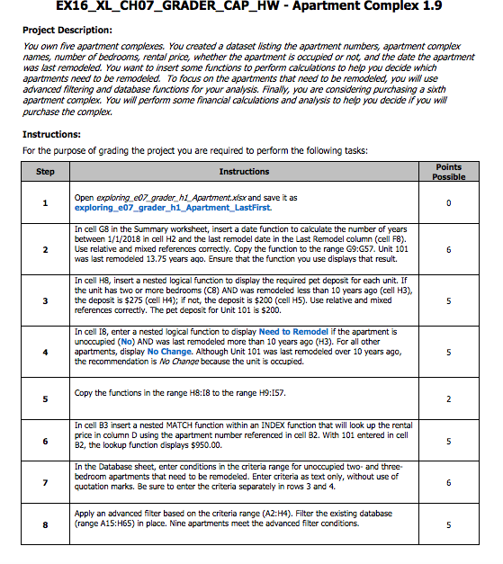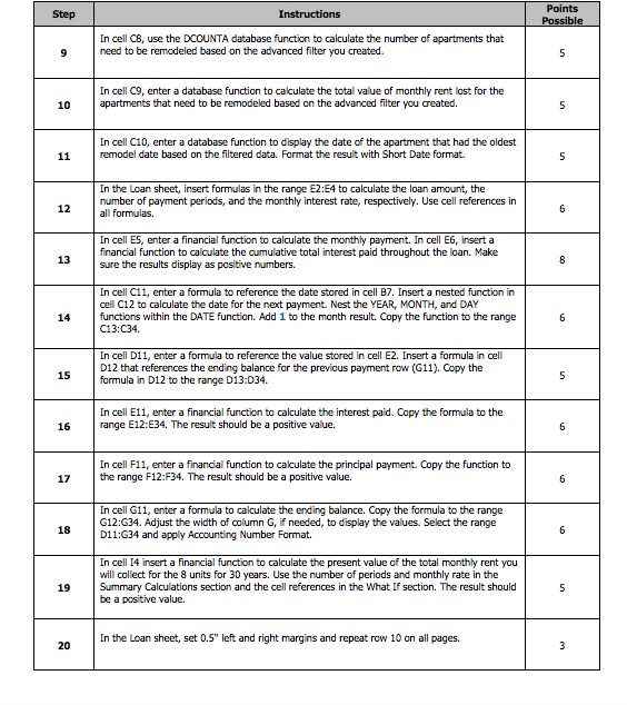


EX16_XL_CH07_GRADER CAP_HW -Apartment Complex 1.9 Project Description: You own five apartment complexes. You created a dataset listing the apartment numbers, apartment complex names, number of bedrooms, rental price, whether the apartment is occupied or not, and the date the apartment was last remodeled You want to insert some functions to perform calculations to help you decide which apartments need to be remodeled. To focus on the apartments that need to be remodeled, you wll use advanced ftering and database functions for your analysis. Finally, you are considering purchasing a sixth apartment complex. You wil perform some financial calculations and analysis to hep you decide if you wl purchase the complex. Instructions: For the purpose of grading the project you are required to perform the following tasks: Points Step Open expioing e07 grader hi Apartmentxisx and save it as In cell G8 in the Summary worksheet, insert a date function to calculate the number of years between 1/1/2018 in cell H2 and the last remodel date in the Last Remodel column (cell F8). Use relative and mixed references correctly. Copy the function to the range G9:G57. Unit 101 was last remodeled 13.75 years ago. Ensure that the function you use displays that result. In cell H8, insert a nested logical function to display the required pet deposit for each unit. If the unit has two or more bedrooms (C8) AND was remodeled less than 10 years ago (cell H3), the deposit is $275 (cell H4); if not, the deposit is $200 (cell HS). Use relative and mixed references correctly. The pet deposit for Unit 101 is $200. In cell I8, enter a nested logical function to display Need to Remodel if the apartment is unoccupied (No) AND was last remodeled more than 10 years ago (H3). For all other apartments, display No Change. Although Unit 101 was last remodeled over 10 years ago, the recommendation is No Change because the unit is occupied. Copy the functions in the range H8:18 to the range H9:I57 In cell B3 insert a nested MATCH function within an INDEX function that will look up the rental price in column D using the apartment number referenced in cell B2. With 101 entered in cell B2, the lookup function displays $950.00. In the Database sheet, enter conditions in the criteria range for unoccupied two- and three- bedroom apartments that need to be remodeled. Enter criteria as text only, without use of quotation marks. Be sure to enter the criteria separately in rows 3 and 4. Apply an advanced filter based on the criteria range (A2:H4). Filter the existing database (range A15:H65) in place. Nine apartments meet the advanced filter conditions. Points Step In cell C8, use the DCOUNTA database function to calculate the number of apartments that need to be remodeled based on the advanced filter you created. In cell C9, enter a database function to calculate the total value of monthly rent lost for the apartments that need to be remodeled based on the advanced filter you created. 10 In cell C10, enter a database function to display the date of the apartment that had the oldest remodel date based on the filtered data. Format the result with Short Date format In the Loan sheet, insert formulas in the range E2:E4 to calculate the loan amount, the number of payment periods, and the monthly interest rate, respectively. Use cell references in all formulas. 12 In cell ES, enter a financial function to calculate the monthly payment. In cell E6, insert a financial function to calculate the cumulative total interest paid throughout the loan. Make sure the results display as positive numbers. In cell C11, enter a formula to reference the date stored in cell B7. Insert a nested function in cel C12 to calculate the date for the next payment. Nest the YEAR, MONTH, and DAY 14 functions within the DATE function. Add 1 to the month result. Copy the function to the range C13:C34 In cell D11, enter a formula to reference the value stored in cell E2. Insert a formula in cell D12 that references the ending balance for the previous payment row (G11). Copy the formula in D12 to the range D13:D34. 15 In cell E11, enter a financial function to calculate the interest paid. Copy the formula to the 16 range E12:E34. The result should be a positive value. In cell F11, enter a financial function to calculate the principal payment. Copy the function to 17 the range F12:F34. The result should be a positive value. In cell G11, enter a formula to calculate the ending balance. Copy the formula to the range G12:G34. Adjust the width of column G, if needed, to display the values. Select the range D11:G34 and apply Accounting Number Format. 18 In cell I4 insert a financial function to calculate the present value of the total monthly rent you will collect for the 8 units for 30 years. Use the number of periods and monthly rate in the 19 Summary Calculations section and the cell references in the What If section. The result should be a positive value. In the Loan sheet, set 0.5" left and right margins and repeat row 10 on all pages. 20 Points Possible Instructions Step 21 Save and close the workbook, and submit the file as directed. Total Points 100


