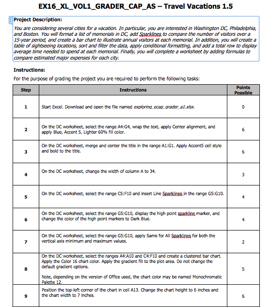
EX16_XL_VOL1_GRADER CAP_AS- Travel Vacations 1.5 Project Description: You are considering several cities for a vacation. In particular, you are interested in Washington DC Phiadephia, and Boston. You will format a list of memonals in Dc, add Soacklines to compare the number of visitors over a 15-year peniod, and create a bar chart to ustrate annual isitors at each memorial. In addition, you will create a table of sightseeing locations, sort and filter the data, apply conditional formatting, and add a total row to display average time needed to spend at each memonal. Finally, you will complete a worksheet by adding formulas to compare estimated major expenses for each city. For the purpose of grading the project you are required to perform the following tasks: Points Step Start Excel. Download and open the file named expornzeca rader a1.mk On the DC worksheet, select the range A4:G4, wrap the text, apply Center alignment, and apply Blue, Accent 5, Lighter 60% fill oolor On the DC worksheet, merge and center the title in the range A1:G1. Apply Accents cell style and bold to the title. On the DC worksheet, change the width of column A to 34. On the DC worksheet, select the range CS:F10 and insert Line Sparkines in the range GS:G10. On the DC worksheet, select the range GS:G10, display the high point spackline marker, and change the color of the high point markers to Dark Blue. On the DC worksheet, select the range G5:G10, apply Same for All Sparklines for both the vertical axis minimum and maximum values. On the DC worksheet, select the ranges A4:A10 and C4:F10 and create a clustered bar chart. Apply the Color 16 chart color. Apply the gradient fill to the plot area. Do not change the default gradient options. Note, depending on the version of Office used, the chart color may be named Monochromatic lette Position the top-left corner of the chart in cell A13. Change the chart height to 6 inches and the chart width to 7 inches. EX16_XL_VOL1_GRADER CAP_AS- Travel Vacations 1.5 Project Description: You are considering several cities for a vacation. In particular, you are interested in Washington DC Phiadephia, and Boston. You will format a list of memonals in Dc, add Soacklines to compare the number of visitors over a 15-year peniod, and create a bar chart to ustrate annual isitors at each memorial. In addition, you will create a table of sightseeing locations, sort and filter the data, apply conditional formatting, and add a total row to display average time needed to spend at each memonal. Finally, you will complete a worksheet by adding formulas to compare estimated major expenses for each city. For the purpose of grading the project you are required to perform the following tasks: Points Step Start Excel. Download and open the file named expornzeca rader a1.mk On the DC worksheet, select the range A4:G4, wrap the text, apply Center alignment, and apply Blue, Accent 5, Lighter 60% fill oolor On the DC worksheet, merge and center the title in the range A1:G1. Apply Accents cell style and bold to the title. On the DC worksheet, change the width of column A to 34. On the DC worksheet, select the range CS:F10 and insert Line Sparkines in the range GS:G10. On the DC worksheet, select the range GS:G10, display the high point spackline marker, and change the color of the high point markers to Dark Blue. On the DC worksheet, select the range G5:G10, apply Same for All Sparklines for both the vertical axis minimum and maximum values. On the DC worksheet, select the ranges A4:A10 and C4:F10 and create a clustered bar chart. Apply the Color 16 chart color. Apply the gradient fill to the plot area. Do not change the default gradient options. Note, depending on the version of Office used, the chart color may be named Monochromatic lette Position the top-left corner of the chart in cell A13. Change the chart height to 6 inches and the chart width to 7 inches