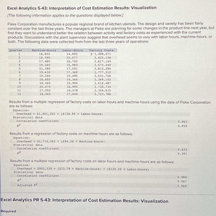
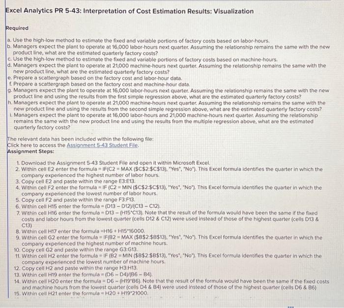
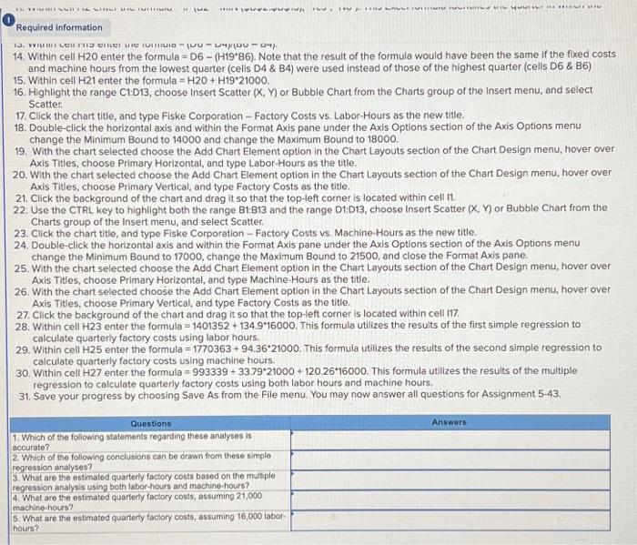
Excel Analytics 5-43: Interpretation of Cost Estimation Results: Visualization [The following information applies to the questions displayed below.] Fiske Corporation manufactures a popular regional brand of kitchen utensils. The design and variety has been fairly constant over the last three years. The managers at Fiske are planning for some changes in the product line next year, but first they want to understand better the relation between activity and factory costs as experienced with the current products. Discussions with the plant supervisor suggest that overhead seems to vary with labor-hours, machine-hours, or both. The following data were collected from from the last three years of operations: Results from a multiple regression of factory costs on labor-hours and machine-hours using the data of Fiske Corporation are as follows: Equation: Overhead =$1,401,352+($134.90 Labor-hours ) Statistical data Correlation coetficient R2 Equation: Overhead =$1,401,352+($134.90 Labor-hours ) Statistical data Correlation coeficient R2 0.963 0.928 Results from a regression of factory costs on machine-hours are as follows: Equation: Overhead =$1,770,363+($94.36 Machine-hours ) Statistical data Correlation coefficient R2 0.625 0.391 Results from a multiple regression of factory costs on labor-hours and machine-hours are as follows: Rquation: Overhead =$993,339+($33.79 Machine-hours )+($120,26 Labor-hours ) Statistical data Correlation coefficient R2 0.984 Adjusted R2 0.967 0.960 Excel Analytics PR 5-43: Interpretation of Cost Estimation Results: Visualization Required Required a. Use the high-low method to estimate the fixed and variable portions of factory costs based on labor-hours. b. Managers expect the plant to operate at 16,000 labor-hours next quarter. Assuming the relationship remains the same with the new product line, what are the estimated quarterly factory costs? c. Use the high-low method to estimate the fixed and variable portions of factory costs based on machine-hours. d. Managers expect the plant to operate at 21,000 machine-hours next quarter. Assuming the relationship remains the same with the new product line, what are the estimated quarterly factory costs? e. Prepare a scattergraph based on the factory cost and labor-hour data. f. Prepare a scattergraph based on the factory cost and machine-hour data. 9. Managers expect the plant to operate at 16,000 labor-hours next quarter. Assuming the relationship remains the same with the new product line and using the results from the first simple regression above, what are the estimated quarterly factory costs? h. Managers expect the plant to operate at 21,000 machine-hours next quarter. Assuming the relationship remains the same with the new product line and using the results from the second simple regression above. what are the estimated quarterly factory costs? 1. Managers expect the plant to operate at 16,000 labor-hours and 21,000 machine-hours next quarter. Assuming the relationship remains the same with the new product line and using the tesults from the multiple regression above, what are the estimated quarterly factory costs? The relevant data has been included within the following file: Click here to access the Assignment 5-43 Student File. Assignment Steps: 1. Download the Assignment 5-43 Student File and open it within Microsoft Excel. 2. Within cell E2 enter the formula = IF(C2 = MAX (\$C\$2:\$C\$13), "Yes", "No"). This Excel formula identifies the quarter in which the company experienced the highest number of labor hours. 3. Copy cell E2 and paste within the range E3:E13. 4. Within cell F2 enter the formula = IF (C2 = MIN (\$C\$2:\$C\$13), 'Yos", "No'), This Excel formula identifies the quarter in which the company experienced the lowest number of labor hours. 5. Copy cell F2 and paste within the range F3 F13. 6. Within cell H15 enter the formula =(D13D12)/(C13C12). 7. Within cell H16 enter the formula =D13(H15C13), Note that the result of the formula would have been the same if the fixed costs and labor hours from the lowest quarter (cells D12 \& C12) were used instead of those of the highest quarter (cells D13 \& C13) 8. Within cell H17 enter the formula =H16+H151600O. 9. Within cell G2 enter the formula = IF(B2 = MAX (\$B\$2\$B\$13), "Yes", "No"). This Excel formula identifies the quarter in which the company experienced the highest number of machine hours. 10. Copy cell G2 and paste within the range G3:G13. company experienced the lowest number of machine hours. 12. Copy cell H2 and paste within the range H3.H13. 13. Within cell H19 enter the formula =(D6D4)/(B6B4). 14. Within cell H2O enter the formula =D6(H19+B). Note that the result of the formula would have been the same if the fixed costs and machine hours from the lowest quarter (cells D4 \& B4) were used instead of those of the highest quarter (cells D6 \& B6) 15. Within cell H21 enter the formula =H2O+H192100O. Required information 14. Within cell H2O enter the formula =D6(H19B6). Note that the result of the formula would have been the same if the fixed costs and machine hours from the lowest quarter (celis D4 \& B4) were used instead of those of the highest quarter (cells D6 \& B6) 15. Within cell H21 enter the formula =H2O+H1921000. 16. Highlight the range C1:D13, choose Insert Scatter (X,Y) or Bubble Chart from the Charts group of the Insert menu, and select Scattet: 17. Click the chart title, and type Fiske Corporation - Factory Costs vs. Labor-Hours as the new title. 18. Double-click the horizontal axis and within the Format Axis pane under the Axis Options section of the Axis Options menu change the Minimum Bound to 14000 and change the Maximum Bound to 18000 . 19. With the chart selected choose the Add Chart Element option in the Chart Layouts section of the Chart Design menu, hover over Axis Titles, choose Primary Horizontal, and type Labor-Hours as the title. 20. With the chart selected choose the Add Chart Element option in the Chart Layouts section of the Chart Design menu, hover over Axis Tites, choose Primary Vertical, and type Factory Costs as the title. 21. Click the background of the chart and drag it so that the top-left corner is located within cell it. 22. Use the CTRL key to highlight both the range B1:B13 and the range D1:D13, choose Insert Scatter (X, Y) or Bubble Chart from the Charts group of the insert menu, and select Scatter. 23. Click the chart title, and type Fiske Corporation - Factory Costs vs. Machine-Hours as the new title. 24. Double-click the horizontal axis and within the Format Axis pane under the Axis Options section of the Axis Options menu change the Minimum Bound to 17000, change the Maximum Bound to 21500, and close the Format Axis pane. 25. With the chart selected choose the Add Chart Element option in the Chart Layouts section of the Chart Design menu, hover over Axis Titles, choose Primary Horizontal, and type Machine-Hours as the title. 26. With the chart selected choose the Add Chart Element option in the Chart Layouts section of the Chart Design menu, hover over Axis Tities, choose Primary Vertical, and type Factory Costs as the title. 27. Click the background of the chart and drag it so that the top-left corner is located within cell 117. 28. Within cell H23 enter the formula =1401352+134.916000. This formula utilizes the results of the first simple regression to calculate quarterly factory costs using labor hours. 29. Within cell H25 enter the formula =1770363+94,3621000. This formula utilizes the results of the second simple regression to caiculate quarterly factory costs using machine hours. 30. Within cell H27 enter the formula =993339+33.7921000+120.2616000. This formula utilizes the results of the multiple regression to calculate quarterly factory costs using both labor hours and machine hours. 31. Save your progress by choosing Save As from the File menu. You may now answer all questions for Assignment 543