Excel Lab:
Please complete this completely. Thanks
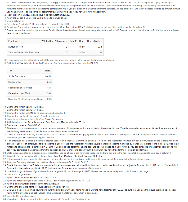
1. To successfully complete this assignment,I strongly recommend that you complete the Excel file in Excel Chapter 3 before you start this assignment. Trying to look up the formulas, cell references, and IF statement while attempting the assignment does not work well unless you understand what you are doing. The best way to understand is to follow the numbered steps in the chapter to complete the file. If you get stuck on the example from the textbook, please email me. I will tell you exactly what to do or what formula you need. I will not do the same for assignments, but I will help you if you have put forth honest effort. 2. Right click on the Lab8 s and save it as YourLastNameLab8. 3. Apply the Depth theme or the Berlin theme to the worksheet 4. Delete column E 5. Set column A width to 31.00, and columns B through K to 11.00. 8. Select row 3 and set text to wrap in this row using the Wrap Text button (HOME tab Alignment group), and then set the row height to best fit. 7. Delete the row that contains the employee Butabi, Steve. Insert two blank lines immediately above the row for Huff, Brennan, and add the information for the two new employees listed in the table below Employee Burgundy, Ron YourLastName, YourFirstName Withholding Allowances Rate Per Hour 16.50 18.00 Hours Worked 32.5 48 8. If necessary, use the fill handle in cell E6 to copy the gross pay formula to the rows of the two new employees. 9. Add the text Tax Rates to the cell A15. Add the Tax Rates information below to cells A18:B20 Rate 0.45% 1.55% 14% Social Security tax Medicare tax Federal tax S889 or less Federal tax over 5689 State tax (% of federal withholding) 24% 20% 10. Change the font in cell A1 to 28-point. 11. Change the font in cell A2 to 18-point. 12. Change the font in cell A15 to 18-point italic and underlined. 13. Change the row height for rows 1, 2, and 15 to best fit. 14. Insert three columns to the right of the Gross Pay column. 15. Add the column titles Taxable Income, Soc. Sec., and Medicare in cells F3:H3 16. Center the contents of cells B3:K3 17. The federal tax calculations must take into account two tiers of income tax, which are applied to the taxable income. Taxable income is caculated as Gross Pay (number of withholding allowances x S90). Be sure to use parentheses as needed. 18. Calculate the Social Security and Medicare taxes in columns G and H by multiplying the tax rates in the Tax Rates table by the Gross Pay. In your formulas, use absolute cel references (like SB516) when using the tax rates. 19. If an employee has a taxable income of greater S689, then the federal tax withheld equals S110.85 plus the federal tax rate found in cell B19 multiplied by the taxable income in excess of S889. If an employees taxable income is S889 or less, the federal tax withheld equals the taxable income multiplied by the federal tax rate found in cell B18. Use the IF function to calculate the Federal Tax in Column I. Be sure to use parentheses and absolute cell references as in your formula. You can email the professor for help, but he will ask if you completed the exercises from the textbook and will want you to attach your file with what you have tried for the IF function and formula. 20. State tax is calculated as a percentage of federal tax. Use an absolute cell reference that uses the State tax rate in the Tax Rates table to calculate state tax in column J 21. Calculate Net Pay in column K, as Gross Pay - Soc. Sec., Medicare, Federal Tax, and State Tax 22. If done correctly, you should be able to enter the formulas for the first employee and then use fill down to find the amounts for the remaining employees. 23. Apply the Currency style with two decimal places to the range C4:C11 and E4:K12. 24. Check the formulas in the Totals row to ensure that all employees are calculated into the totals. I had to use AutoSum and adjust the formulas in 112, J12, and K12 when I did it Ensure that the total net pay is $4,187.80. Include totals for the amounts in columns D through K. 25. Use the background color of your choice for the range A1:K2, and the range A15:B20. Please use the same background color for each cell range. 26. Center the range B4:811 27. Apply a Thick Bottom Border to the range A3:K3. 28. Apply the Total cell style to the range A12:K12. Set the row height of row 12 to 17.25. 29. Apply a Thick Outside Border to the range A15:B20 30. Change the sheet tab name to YourLastName-Weekly Payroll. 31. Use Goal Seek to determine how many hours the employee with your name needs to work to have Net Pay of $700.00 (be sure that you use the Hours Worked cell for your name for the By changing cell: val This will revise the total net pay, which is acceptable 32. Save the file and close Excel 33. Upload and submit the completed file to the appropriate Desire2Learn Dropbox folder 1. To successfully complete this assignment,I strongly recommend that you complete the Excel file in Excel Chapter 3 before you start this assignment. Trying to look up the formulas, cell references, and IF statement while attempting the assignment does not work well unless you understand what you are doing. The best way to understand is to follow the numbered steps in the chapter to complete the file. If you get stuck on the example from the textbook, please email me. I will tell you exactly what to do or what formula you need. I will not do the same for assignments, but I will help you if you have put forth honest effort. 2. Right click on the Lab8 s and save it as YourLastNameLab8. 3. Apply the Depth theme or the Berlin theme to the worksheet 4. Delete column E 5. Set column A width to 31.00, and columns B through K to 11.00. 8. Select row 3 and set text to wrap in this row using the Wrap Text button (HOME tab Alignment group), and then set the row height to best fit. 7. Delete the row that contains the employee Butabi, Steve. Insert two blank lines immediately above the row for Huff, Brennan, and add the information for the two new employees listed in the table below Employee Burgundy, Ron YourLastName, YourFirstName Withholding Allowances Rate Per Hour 16.50 18.00 Hours Worked 32.5 48 8. If necessary, use the fill handle in cell E6 to copy the gross pay formula to the rows of the two new employees. 9. Add the text Tax Rates to the cell A15. Add the Tax Rates information below to cells A18:B20 Rate 0.45% 1.55% 14% Social Security tax Medicare tax Federal tax S889 or less Federal tax over 5689 State tax (% of federal withholding) 24% 20% 10. Change the font in cell A1 to 28-point. 11. Change the font in cell A2 to 18-point. 12. Change the font in cell A15 to 18-point italic and underlined. 13. Change the row height for rows 1, 2, and 15 to best fit. 14. Insert three columns to the right of the Gross Pay column. 15. Add the column titles Taxable Income, Soc. Sec., and Medicare in cells F3:H3 16. Center the contents of cells B3:K3 17. The federal tax calculations must take into account two tiers of income tax, which are applied to the taxable income. Taxable income is caculated as Gross Pay (number of withholding allowances x S90). Be sure to use parentheses as needed. 18. Calculate the Social Security and Medicare taxes in columns G and H by multiplying the tax rates in the Tax Rates table by the Gross Pay. In your formulas, use absolute cel references (like SB516) when using the tax rates. 19. If an employee has a taxable income of greater S689, then the federal tax withheld equals S110.85 plus the federal tax rate found in cell B19 multiplied by the taxable income in excess of S889. If an employees taxable income is S889 or less, the federal tax withheld equals the taxable income multiplied by the federal tax rate found in cell B18. Use the IF function to calculate the Federal Tax in Column I. Be sure to use parentheses and absolute cell references as in your formula. You can email the professor for help, but he will ask if you completed the exercises from the textbook and will want you to attach your file with what you have tried for the IF function and formula. 20. State tax is calculated as a percentage of federal tax. Use an absolute cell reference that uses the State tax rate in the Tax Rates table to calculate state tax in column J 21. Calculate Net Pay in column K, as Gross Pay - Soc. Sec., Medicare, Federal Tax, and State Tax 22. If done correctly, you should be able to enter the formulas for the first employee and then use fill down to find the amounts for the remaining employees. 23. Apply the Currency style with two decimal places to the range C4:C11 and E4:K12. 24. Check the formulas in the Totals row to ensure that all employees are calculated into the totals. I had to use AutoSum and adjust the formulas in 112, J12, and K12 when I did it Ensure that the total net pay is $4,187.80. Include totals for the amounts in columns D through K. 25. Use the background color of your choice for the range A1:K2, and the range A15:B20. Please use the same background color for each cell range. 26. Center the range B4:811 27. Apply a Thick Bottom Border to the range A3:K3. 28. Apply the Total cell style to the range A12:K12. Set the row height of row 12 to 17.25. 29. Apply a Thick Outside Border to the range A15:B20 30. Change the sheet tab name to YourLastName-Weekly Payroll. 31. Use Goal Seek to determine how many hours the employee with your name needs to work to have Net Pay of $700.00 (be sure that you use the Hours Worked cell for your name for the By changing cell: val This will revise the total net pay, which is acceptable 32. Save the file and close Excel 33. Upload and submit the completed file to the appropriate Desire2Learn Dropbox folder