Excel Lab:
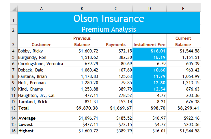
The first table is the completed version.
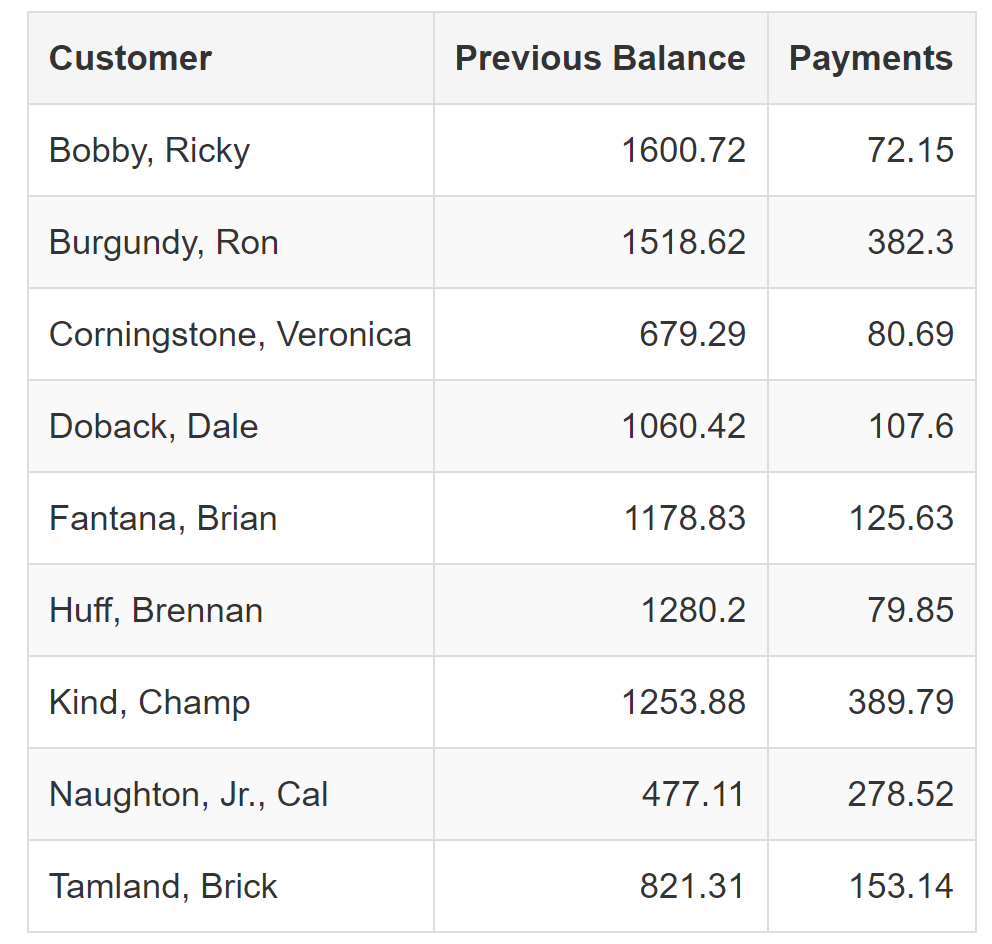
The second table is used at STEP 19.
Please complete this completely. Thanks
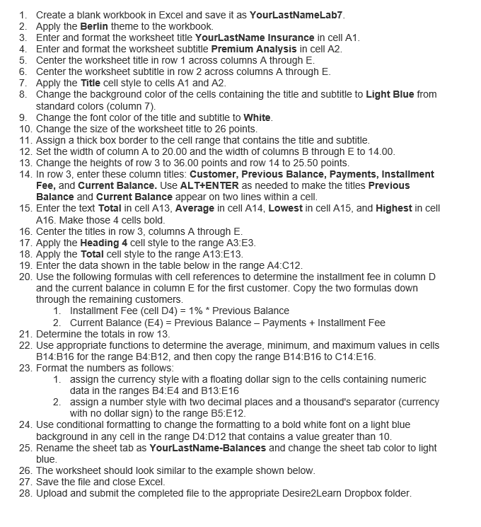
1. Create a blank workbook in Excel and save it as YourLastNameLab7 2. Apply the Berlin theme to the workbook. 3. Enter and format the worksheet title YourLastName Insurance in cell A1 4. Enter and format the worksheet subtitle Premium Analysis in cell A2 5. Center the worksheet title in row 1 across columns A through E. 6. Center the worksheet subtitle in row 2 across columns A through E. 7. Apply the Title cell style to cells A1 and A2 8. Change the background color of the cells containing the title and subtitle to Light Blue from standard colors (column 7) 9. Change the font color of the title and subtitle to White 10. Change the size of the worksheet title to 26 points 11. Assign a thick box border to the cell range that contains the title and subtitle 12. Set the width of column A to 20.00 and the width of columns B through E to 14.00 13. Change the heights of roW 3 to 36.00 points and row 14 to 25.50 points 14. In row 3, enter these column titles: Customer, Previous Balance, Payments, Installment Fee, and Current Balance. Use ALT+ENTER as needed to make the titles Previous Balance and Current Balance appear on two lines within a cell 15. Enter the text Total in cell A13, Average in cell A14, Lowest in cell A15, and Highest in cell A16. Make those 4 cells bold 16. Center the titles in row 3, columns A through E. 17. Apply the Heading 4 cell style to the range A3 E3 18. Apply the Total cell style to the range A13 E13 19. Enter the data shown in the table below in the range A4:C12 20. Use the following formulas with cell references to determine the installment fee in column D and the current balance in column E for the first customer. Copy the two formulas down through the remaining customers 1. 2. Installment Fee (cell D4) 1% * Previous Balance Current Balance (E4) = Previous Balance-Payments + Installment Fee 21. Determine the totals in roW 13 22. Use appropriate functions to determine the average, minimum, and maximum values in cells B14:B16 for the range B4:B12, and then copy the range B14:B16 to C14 E16 23. Format the numbers as follows 1 assign the currency style with a floating dollar sign to the cells containing numeric data in the ranges B4 E4 and B13 E16 2. assign a number style wth two decimal places and a thousand's separator (currency with no dollar sign) to the range B5:E12 24. Use conditional formatting to change the formatting to a bold white font on a light blue background in any cell in the range D4 D12 that contains a value greater than 10 25. Rename the sheet tab as YourLastName-Balances and change the sheet tab color to light blue 26. The worksheet should look similar to the example shown below 27. Save the file and close Excel 28. Upload and submit the completed file to the appropriate Desire2Learn Dropbox folder 1. Create a blank workbook in Excel and save it as YourLastNameLab7 2. Apply the Berlin theme to the workbook. 3. Enter and format the worksheet title YourLastName Insurance in cell A1 4. Enter and format the worksheet subtitle Premium Analysis in cell A2 5. Center the worksheet title in row 1 across columns A through E. 6. Center the worksheet subtitle in row 2 across columns A through E. 7. Apply the Title cell style to cells A1 and A2 8. Change the background color of the cells containing the title and subtitle to Light Blue from standard colors (column 7) 9. Change the font color of the title and subtitle to White 10. Change the size of the worksheet title to 26 points 11. Assign a thick box border to the cell range that contains the title and subtitle 12. Set the width of column A to 20.00 and the width of columns B through E to 14.00 13. Change the heights of roW 3 to 36.00 points and row 14 to 25.50 points 14. In row 3, enter these column titles: Customer, Previous Balance, Payments, Installment Fee, and Current Balance. Use ALT+ENTER as needed to make the titles Previous Balance and Current Balance appear on two lines within a cell 15. Enter the text Total in cell A13, Average in cell A14, Lowest in cell A15, and Highest in cell A16. Make those 4 cells bold 16. Center the titles in row 3, columns A through E. 17. Apply the Heading 4 cell style to the range A3 E3 18. Apply the Total cell style to the range A13 E13 19. Enter the data shown in the table below in the range A4:C12 20. Use the following formulas with cell references to determine the installment fee in column D and the current balance in column E for the first customer. Copy the two formulas down through the remaining customers 1. 2. Installment Fee (cell D4) 1% * Previous Balance Current Balance (E4) = Previous Balance-Payments + Installment Fee 21. Determine the totals in roW 13 22. Use appropriate functions to determine the average, minimum, and maximum values in cells B14:B16 for the range B4:B12, and then copy the range B14:B16 to C14 E16 23. Format the numbers as follows 1 assign the currency style with a floating dollar sign to the cells containing numeric data in the ranges B4 E4 and B13 E16 2. assign a number style wth two decimal places and a thousand's separator (currency with no dollar sign) to the range B5:E12 24. Use conditional formatting to change the formatting to a bold white font on a light blue background in any cell in the range D4 D12 that contains a value greater than 10 25. Rename the sheet tab as YourLastName-Balances and change the sheet tab color to light blue 26. The worksheet should look similar to the example shown below 27. Save the file and close Excel 28. Upload and submit the completed file to the appropriate Desire2Learn Dropbox folder