[EXCEL]
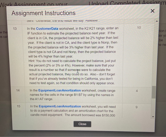
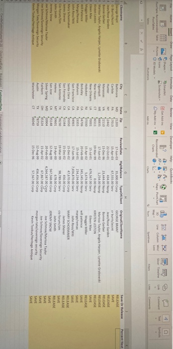
Please help this is the hardest exam I have ever taken in my life. I have been stuck on thirteen for over an hour. I think it is a nested IF function or an IFS function but everything I try is an error.

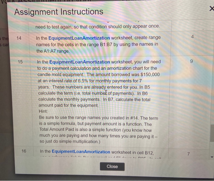
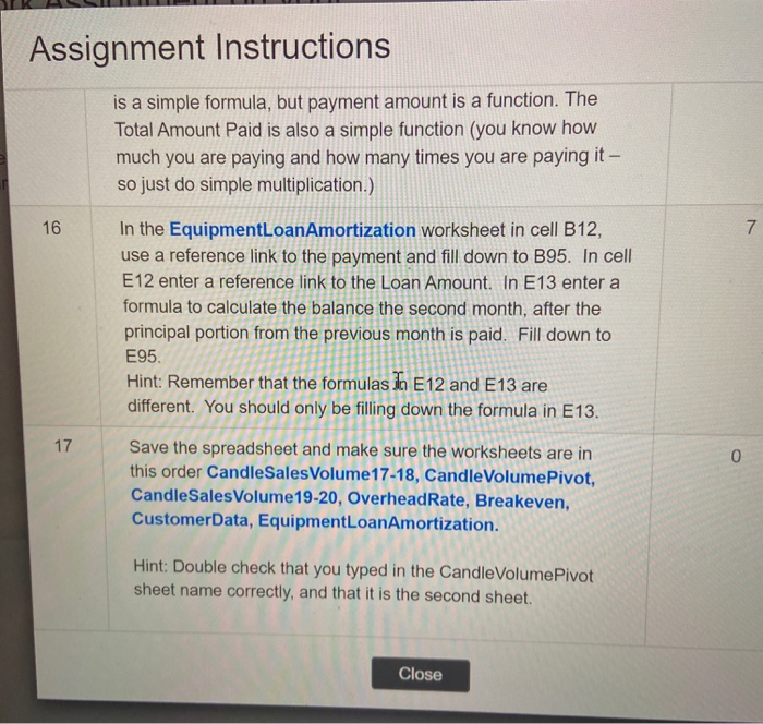
Work Assignment on your I Inload Comnleted Assianm Assignment Instructions selv. Omer wise, we nu result WIII Say Release. 13 10 w the tion ler ya be es car he ne In the CustomerData worksheet, in the K2:K21 range, enter an IF function to estimate the projected balance next year. If the client is in CA, the projected balance will be 2% higher than last year. If the client is not in CA, and the client type is Nonp, then the projected balance will be 3% higher than last year. If the client type is not CA and not Nonp, then the projected balance will be 4% higher than last year. Hint: You do not need to calculate the project balance, just put the percent (2% or 3% or 4%). However, make sure that your result is a number so that if someone were to calculate the actual projected balance, they could do so. Also - don't forget that if you've already tested for being in California, you don't need to test again, so that condition should only appear once. 14 4 In the EquipmentLoanAmortization worksheet, create range names for the cells in the range B1:B7 by using the names in the A1:A7 range. 15 9 In the EquipmentLoanAmortization worksheet, you will need to do a payment calculation and an amortization chart for the candle mold equipment. The amount borrowed was $150,000 Close Assignment Instructions 14 4 the scar 15 9 need to test again, so that condition should only appear once. In the EquipmentLoanAmortization worksheet, create range names for the cells in the range B1:B7 by using the names in the A1:A7 range. In the EquipmentLoanAmortization worksheet, you will need to do a payment calculation and an amortization chart for the candle mold equipment. The amount borrowed was $150,000 at an interest rate of 6.5% for monthly payments for 7 years. These numbers are already entered for you. In B5 calculate the term (i.e. total numbel of payments). In B6 calculate the monthly payments. In B7, calculate the total amount paid for the equipment. Hint: Be sure to use the range names you created in #14. The term is a simple formula, but payment amount is a function. The Total Amount Paid is also a simple function (you know how much you are paying and how many times you are paying it - so just do simple multiplication.) In the EquipmentLoanAmortization worksheet in cell B12, 16 Close Assignment Instructions is a simple formula, but payment amount is a function. The Total Amount Paid is also a simple function (you know how much you are paying and how many times you are paying it - so just do simple multiplication.) 16 7 In the EquipmentLoanAmortization worksheet in cell B12, use a reference link to the payment and fill down to B95. In cell E12 enter a reference link to the Loan Amount. In E13 enter a formula to calculate the balance the second month, after the principal portion from the previous month is paid. Fill down to E95 Hint: Remember that the formulas in E12 and E13 are different. You should only be filling down the formula in E13. 17 0 Save the spreadsheet and make sure the worksheets are in this order CandleSalesVolume17-18, CandleVolumePivot, CandleSalesVolume 19-20, OverheadRate, Breakeven, CustomerData, EquipmentLoanAmortization. Hint: Double check that you typed in the Candle VolumePivot sheet name correctly, and that it is the second sheet. Close Home D Page Layout Formas Data Review View Developer He - P-75 es 4 C Get Ad uy Add FD Maps Potchat hun spmbols Link Recommended Charts Line Column Way Los Petables Map Charts Linas fe Percent Next Save Or Release RELEASE SAVE 1 Clentname George Brant 3 O Burris/Acet Jean Rose Garden 5 Bonnie Gerber 6 Mar Taylor Angel Harper, Lynette Grabowski "Yol City State Zip atimore MD 21203 Care PA 17011 Hunter NY 12442 Mansas VA 22110 Opungut ME RRUS New Haven CT New Orleans LA Hoboken NI 010 Berkeley CA 54700 Malver PA 19355 San Francisco CA Santa Clara CA CA 91144 San Antonio 78230 Helena MT S90 San Jose CA 55145 Silver Spring MD 20904 Fairbom OH 45334 Austin TX 78750 Manchester CT 1040 en Max - Ma Me w Patience 1 Margemas 2 John Row 3 Mary Schoemaker 4 lames Shener 5 Co Fourim 6 John Smith 7 Jeremy now Joe Schoe/Marisa Taylor 9 Joe Schmoovereign Security Morgan Tate/Soverei Security 1 Kevin Took/Heritage Antique ReviewDate High Balance TypeOlent 17.03 35,000 00 Corp 15 or 01 6755500 Ser 22-Oct-01 43400 Non 15-Dec. 23.41400 Nonp 17.Jun 02 1,25400 None 19 Mart 000 Non 15-11-01 676.56700 Ser 15 Apr 02 5,67400 Serv 20 Feb 00 345,345.00 NORD 15 Jul-01 234 23400 Serv 17 Jun96 7,656,870 00 Serv 15 Dec 02 47,670 00 Corp 15 Dec 456 00 Corp 19-Mar-29 98,789.00 Serv 19-Apr-00 678.00 Corp 12 Aug 99 567,568.00 Corp 20-Feb-00 4,564,58700 Corp 15 Aro 67,867.00 Corp 12-Aug-99 456,456.00 COP 15-Dec-96 57,567.00 Corp Originaliame GEORGE BRANT crburscent Jean Rose Garden Bonnie Gerber Marisa Taylor, Angela Harper Lette Grabowski KIRSTEN LESTON Teen Max Mace Miller will patience mars/remax John Rossi MARY SCHOEMAKER James Shener cioforum/sim John Smith JEREMY SNOW Joe Schme/Marisa Taylor Joe Schmoe/Sovereign Security morgan tatovereign security Kevin Tooks/Heritage Antique RELEASE RELEASE RELEASE RELEASE SAVE RELEASE SAVE SAVE SAVE RELEASE RELEASE SAVE RELEASE sos SAVE SAVE SAVE SAVE SAVE Cand volume 19:20 Work Assignment on your I Inload Comnleted Assianm Assignment Instructions selv. Omer wise, we nu result WIII Say Release. 13 10 w the tion ler ya be es car he ne In the CustomerData worksheet, in the K2:K21 range, enter an IF function to estimate the projected balance next year. If the client is in CA, the projected balance will be 2% higher than last year. If the client is not in CA, and the client type is Nonp, then the projected balance will be 3% higher than last year. If the client type is not CA and not Nonp, then the projected balance will be 4% higher than last year. Hint: You do not need to calculate the project balance, just put the percent (2% or 3% or 4%). However, make sure that your result is a number so that if someone were to calculate the actual projected balance, they could do so. Also - don't forget that if you've already tested for being in California, you don't need to test again, so that condition should only appear once. 14 4 In the EquipmentLoanAmortization worksheet, create range names for the cells in the range B1:B7 by using the names in the A1:A7 range. 15 9 In the EquipmentLoanAmortization worksheet, you will need to do a payment calculation and an amortization chart for the candle mold equipment. The amount borrowed was $150,000 Close Assignment Instructions 14 4 the scar 15 9 need to test again, so that condition should only appear once. In the EquipmentLoanAmortization worksheet, create range names for the cells in the range B1:B7 by using the names in the A1:A7 range. In the EquipmentLoanAmortization worksheet, you will need to do a payment calculation and an amortization chart for the candle mold equipment. The amount borrowed was $150,000 at an interest rate of 6.5% for monthly payments for 7 years. These numbers are already entered for you. In B5 calculate the term (i.e. total numbel of payments). In B6 calculate the monthly payments. In B7, calculate the total amount paid for the equipment. Hint: Be sure to use the range names you created in #14. The term is a simple formula, but payment amount is a function. The Total Amount Paid is also a simple function (you know how much you are paying and how many times you are paying it - so just do simple multiplication.) In the EquipmentLoanAmortization worksheet in cell B12, 16 Close Assignment Instructions is a simple formula, but payment amount is a function. The Total Amount Paid is also a simple function (you know how much you are paying and how many times you are paying it - so just do simple multiplication.) 16 7 In the EquipmentLoanAmortization worksheet in cell B12, use a reference link to the payment and fill down to B95. In cell E12 enter a reference link to the Loan Amount. In E13 enter a formula to calculate the balance the second month, after the principal portion from the previous month is paid. Fill down to E95 Hint: Remember that the formulas in E12 and E13 are different. You should only be filling down the formula in E13. 17 0 Save the spreadsheet and make sure the worksheets are in this order CandleSalesVolume17-18, CandleVolumePivot, CandleSalesVolume 19-20, OverheadRate, Breakeven, CustomerData, EquipmentLoanAmortization. Hint: Double check that you typed in the Candle VolumePivot sheet name correctly, and that it is the second sheet. Close Home D Page Layout Formas Data Review View Developer He - P-75 es 4 C Get Ad uy Add FD Maps Potchat hun spmbols Link Recommended Charts Line Column Way Los Petables Map Charts Linas fe Percent Next Save Or Release RELEASE SAVE 1 Clentname George Brant 3 O Burris/Acet Jean Rose Garden 5 Bonnie Gerber 6 Mar Taylor Angel Harper, Lynette Grabowski "Yol City State Zip atimore MD 21203 Care PA 17011 Hunter NY 12442 Mansas VA 22110 Opungut ME RRUS New Haven CT New Orleans LA Hoboken NI 010 Berkeley CA 54700 Malver PA 19355 San Francisco CA Santa Clara CA CA 91144 San Antonio 78230 Helena MT S90 San Jose CA 55145 Silver Spring MD 20904 Fairbom OH 45334 Austin TX 78750 Manchester CT 1040 en Max - Ma Me w Patience 1 Margemas 2 John Row 3 Mary Schoemaker 4 lames Shener 5 Co Fourim 6 John Smith 7 Jeremy now Joe Schoe/Marisa Taylor 9 Joe Schmoovereign Security Morgan Tate/Soverei Security 1 Kevin Took/Heritage Antique ReviewDate High Balance TypeOlent 17.03 35,000 00 Corp 15 or 01 6755500 Ser 22-Oct-01 43400 Non 15-Dec. 23.41400 Nonp 17.Jun 02 1,25400 None 19 Mart 000 Non 15-11-01 676.56700 Ser 15 Apr 02 5,67400 Serv 20 Feb 00 345,345.00 NORD 15 Jul-01 234 23400 Serv 17 Jun96 7,656,870 00 Serv 15 Dec 02 47,670 00 Corp 15 Dec 456 00 Corp 19-Mar-29 98,789.00 Serv 19-Apr-00 678.00 Corp 12 Aug 99 567,568.00 Corp 20-Feb-00 4,564,58700 Corp 15 Aro 67,867.00 Corp 12-Aug-99 456,456.00 COP 15-Dec-96 57,567.00 Corp Originaliame GEORGE BRANT crburscent Jean Rose Garden Bonnie Gerber Marisa Taylor, Angela Harper Lette Grabowski KIRSTEN LESTON Teen Max Mace Miller will patience mars/remax John Rossi MARY SCHOEMAKER James Shener cioforum/sim John Smith JEREMY SNOW Joe Schme/Marisa Taylor Joe Schmoe/Sovereign Security morgan tatovereign security Kevin Tooks/Heritage Antique RELEASE RELEASE RELEASE RELEASE SAVE RELEASE SAVE SAVE SAVE RELEASE RELEASE SAVE RELEASE sos SAVE SAVE SAVE SAVE SAVE Cand volume 19:20
