Excel Project $2$: Amortization of the loan.

Exercise

In the Excel file "YourNameProject$2"$ create a copy of Example worksheet $($right click on the

worksheet name on the bottom, select Move or Copy, create a copy$),$ and rename it to Exercise.

Suppose that you have the credit card balance of $$3800\mathrm{.}00$ at the annual interest rate of $17\mathrm{.}55\%$

compounded monthly. You decided that you will not charge anything else to this account and will create

an "amortization schedule" for paying off your dept. You could create the different payment plans.

PAYMENT PLAN $1$:

Enter the following data for the payment plan $1$: $P=3800,r=0\mathrm{.}1755,m=12$

$($change the existing Example data$)$

You are committed to paying off this debt in $3$ years $($or in exactly $36$ payments$).$

Step $1$: Compute the monthly payment so that the debt is amortized $($paid off$)$ at the end of $3$ years.

Step $2$: Create the amortization table through $36$ payments.

Step $3$: Calculate how much you actually paid over the life of the loan and how much interest you paid.

PAYMENT PLAN $2$:

Enter the following data for the payment plan $2$: $P=3800,r=0\mathrm{.}1755,m=12$

$($change the existing Example data$)$

Assume that for the first $36$ months you will pay only the minimum amount required.

The minimum payment due is $2\%$ of the remaining balance.

Step $4$: Create the amortization table through the first $36$ payments and calculate in C$124$ how much

you actually paid over the first $36$ months.

Step $5$:

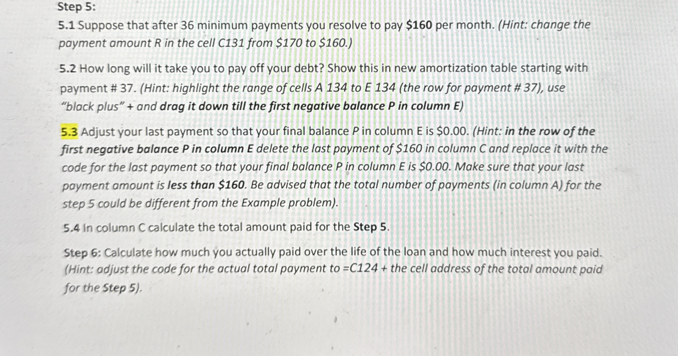
$5\mathrm{.}1$ Suppose that after $36$ minimum payments you resolve to pay $$160$ per month. $($Hint: change the

payment amount $R$ in the cell C$131$ from $$170$ to $$160.)$

$5\mathrm{.}2$ How long will it take you to pay off your debt? Show this in new amortization table starting with

payment # $37.($Hint: highlight the range of cells A $134$ to E $134($the row for payment # $37),$ use

"black plus" $+$ and drag it down till the first negative balance $P$ in column E$)$

$5\mathrm{.}3$ Adjust your last payment so that your final balance $P$ in column E is $$0\mathrm{.}00.($Hint: in the row of the

first negative balance P in column E delete the last payment of $$160$ in column $C$ and replace it with the

code for the last payment so that your final balance P in column E is $$0\mathrm{.}00.$ Make sure that your last

payment amount is less than $$160.$ Be advised that the total number of payments $($in column $A)$ for the

step $5$ could be different from the Example problem$).$

$5\mathrm{.}4$ in column C calculate the total amount paid for the Step $5.$

Step $6$: Calculate how much you actually paid over the life of the loan and how much interest you paid.

$($Hint: adjust the code for the actual total payment to $=C124+$ the cell address of the total amount paid

for the Step $5).$