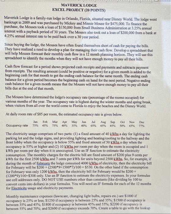
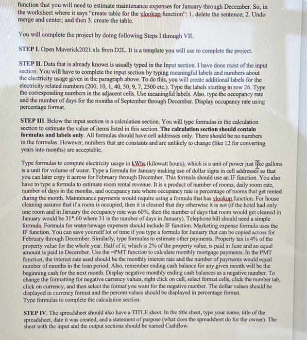
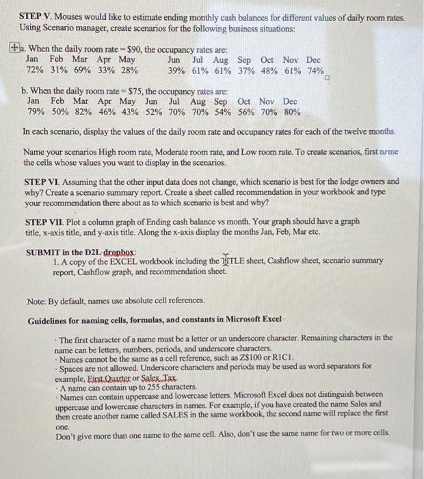
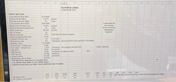
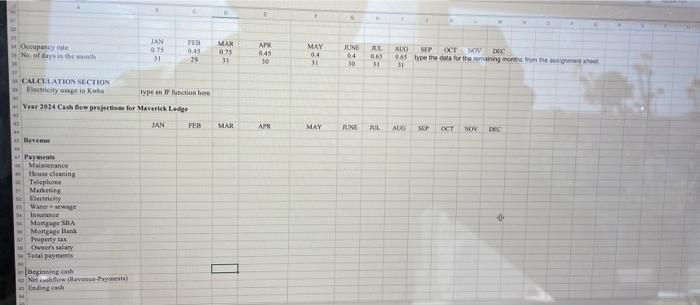
EXCEL PROJECT (20 POINTS) Maverick Lodge is a family-run lodge in Orlando, Florida, situated near Disney World. The lodge went bankrupt in 2009 and was purchased by Mickey and Minnie Mouse for \$475,000. To finance the purchase, the Mouses took a loan of $150,000 from Small Business Administration at 3.25% annual interest with a payback period of 30 years. The Mouses also took out a loan of $200,000 from a bank at 4.25% annual interest rate to be paid back over a 30 year period. Since buying the lodge, the Mouses have often found themselves short of cash for paying the bills. They have realized a need to develop a plan for managing their cash flow. Develop a spreadsheet that will help Mouses forecast their monthly cash flow in a 12 month planning horizon. They will use this spreadsheet to identify the months when they will not have enough moncy to pay all their bills. Cash flow forecast for a period shows projected cash receipts and payments and subtracts payment from receipts. The resulting amount (could be positive or negative) for a given month is added to the beginning cash for that month to get the ending cash balance for the same month. The ending cash balance for a given period becomes the beginning cash on hand for the next period. Negative ending cash balance for a given month means that the Mouses will not have enough moncy to pay all their bills due at the end of that month. The Mouses have determined the lodge's occupancy rate (percentage of the rooms occupied) for various months of the year. The occupancy rate is highest during the winter months and spring break, when visitors from all over the world come to Florida to enjoy the beaches and the Disney World. At daily room rate of $85 per room, the estimated occupancy rate is given below. The electricity usage comprises of two parts: (1) a fixed amount of 40kWhh a day for lighting the parking lot and the lodge signs, and providing lighting and heating/cooling to the hallway and the front lobby when the occupancy is below 55% and fixed amount of 50kWh s a day when the occupancy is 55% or higher and (2) 10 kWblusper room per day when the room is occupied and 1 kWh per room per day when it is unoccupied. Use an IF function to estimate the electricity consumption. The monthly charges for the electric bill are fixed amount of $200 plus 9 cents per kWh for the first 2500kWh and 7 cents per kWh for units beyond 2500kWOh, So, for example, if during the month of Eebnuary the lodge consumed 4000kWh. of electricity, then the electricity bill for February will be $200+(25009+15007)/100=$530. On the other hand if the consumption for February was only 1200 kWbos, then the electricity bill for February would be $200+ (12009)/100=$308 only. Use an IF function to estimate the electricity expenses. In your formulas use cell addresses only. DO NOT USE numbers other than constants (like dividing by 100 to convert cents into dollars) in your formulas. You will need an IF formula for each of the 12 months for Electricity usage and electricity payments. Monthly maintenance expenses (lawncare, changing light bulbs, repairs etc.) are $1000 if function that you will need to estimate maintenance expenses for January through December. So, in the worksheet where it says "create table for the ylookup function": 1 . delete the sentence; 2. Undo merge and center; and then 3 , create the table. You will complete the project by doing following Steps I through VII. STEP I. Open Maverick2021 xls from D2L. It is a template you will use to complete the project. STEP II. Data that is already known is usually typed in the Input section. I have done most of the input section. You will have to complete the input section by typing meaningful labels and numbers about the electricity usage given in the paragraph above. To do this, you will create additional labels for the electricity related numbers (200,10,1,40,50,9,7,2500 etc.). Type the labels starting in row 26 . Type the corresponding numbers in the adjacent cells. Use meaningful labels. Also, type the occupancy rate and the number of days for the months of September through December. Display occupancy rate using percentage format. STEP III. Below the input section is a calculation section. You will type formulas in the calculation section to estimate the value of items listed in this section. The calculation section should contain formulas and labels only. All formulas should have cell addresses only. There should be no numbers in the formulas. However, numbers that are constants and are unlikely to change (like 12 for converting years into months) are acceptable. Type formulas to compute electricity usage in kWbs (kilowatt hours), which is a unit of power just ke gallons is a unit for volume of water. Type a formula for January making use of dollar signs in cell addresses so that you can later copy it across for February through December. This formula should use an IF function. You also have to type a formula to estimate room rental revenue. It is a product of number of rooms, daily room rate, number of days in the months, and occupancy rate where occupancy rate is percentage of rooms that get rented during the month. Maintenance payments would require using a formula that has slookup function. For house cleaning assume that if a room is occupied, then it is cleaned that day otherwise it is not (if the hotel had only one room and in January the occupancy rate was 60%, then the number of days that room would get cleaned in January would be 31.60 where 31 is the number of days in January). Telephone bill should need a simple formula. Formula for water/sewage expenses should include IF function. Marketing expense formula uses the IF function. You can save yourself lot of time if you type a formula for January that can be copied across for February through December. Similarly, type formulas to estimate other payments. Property tax is 4% of the property value for the whole year. Half of it, which is 2% of the property value, is paid in June and an equal amount is paid in December. Use the =PMT function to calculate monthly mortgage payments. In the PMT function, the interest rate used should be the monthly interest rate and the number of payments would equal number of months in the loan period. Also, remember ending cash balance for any given month will be the beginning cash for the next month. Display negative monthly ending cash balances as a negative number. To change the formatting for negative currency values, right click on cell, select format cells, click the number tab, click on currency, and then select the format you want for the negative number. The dollar values should be displayed in currency format and the percent values should be displayed in percentage format. Type formulas to complete the calculation section. STE.P IV. The spreadsheet should also have a TITLE sheet. In the title sheet, type your name, title of the spreadsheet, date it was created, and a statement of purpose (what does the spreadsheet do for the owner). The sheet with the input and the output sections should be named Cashflow. STEP V. Mouses would like to estimate ending monthly cash balances for different values of daily room rates. Using Scenario manager, create scenarios for the following business situations: b. When the daily room rate =$75, the occupancy rates are: In each scenario, display the values of the daily room rate and occupancy rates for each of the twelve months. Name your scenarios High room rate, Moderate room rate, and Low room rate. To create scenarios, first neme the cells whose values you want to display in the scenarios. STEP VL. Assuming that the other input data does not change, which scenario is best for the lodge owners and why? Create a scenario summary report. Create a sheet called recommendation in your workbook and type your recommendation there about as to which scenario is best and why? STEP VII. Plot a column graph of Ending cash balance vs month. Your graph should have a graph title, x-axis title, and y-axis title. Along the x-axis display the months Jan, Feb, Mar etc. SUBMIT in the D2L dropbox: 1. A copy of the EXCEL workbook including the JITLE sheet, Cashflow sheet, scenario summary report, Cashflow graph, and recommendation sheet. Note: By default, names use absolute cell references. Guidelines for naming cells, formulas, and constants in Microsoft Excel - The first character of a name must be a letter or an underscore character. Remaining characters in the name can be letters, numbers, periods, and underscore characters. names cannot be the same as a cell reference, such as ZS100 or RICl. - Spaces are not allowed. Underscore characters and periods may be used as word separators for example, Eirst Quartex or Sales.Tax. A name can contain up to 255 characters. - Names can contain uppercase and lowercase letters. Microsoft Excel does not distinguish between uppercase and lowercase chancters in names. For example, if you have created the name Sales and then create another name called SALES in the same workbook, the second name will replace the first one. Don't give more than one name to the same cell. Also, don't use the same name for two or more cells
