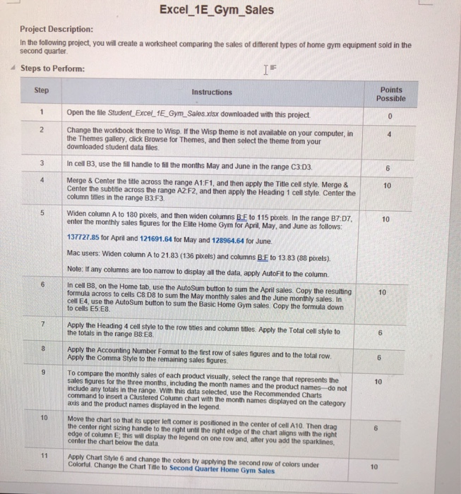
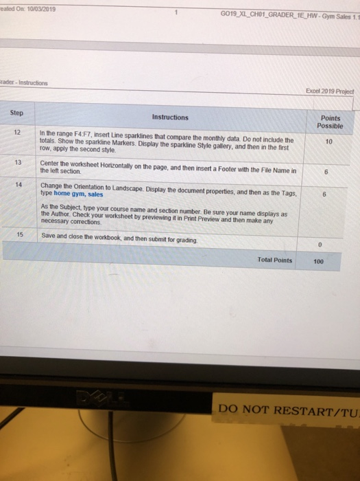
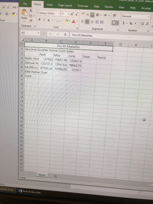
Excel_1E_Gym_Sales Project Description: In the following project, you will create a worksheet comparing the sales of different types of home gym equipment sold in the second quarter IF Steps to Perform: Points Possible Step Instructions Open the file Student Excel 1E Gym Sales xlsx downloaded with this project Change the workbook theme to Wisp. If the Wisp theme is not available on your computer, in the Themes gallery, click Browse for Themes, and then select the theme from your downloaded student data files In cell B3, use the fill handle to fill the months May and June in the range C3.03 Merge & Center the title across the range A1 F1, and then apply the Title cell style. Merge & Center the subtitle across the range A2 F2, and then apply the Heading 1 cell style. Center the column titles in the range B3:F3 Widen column A to 180 pixels, and then widen columns B.E to 115 pixels. In the range B7D7 enter the monthly sales figures for the Elite Home Gym for April, May, and June as follows: 137727.85 for April and 121691.64 for May and 128964.64 for June. Mac users: Widen column A to 21.83 (136 pixels) and columns B.E to 13.83 (88 povels). Note: If any columns are too narrow to display all the data, apply AutoFit to the column In cell B8, on the Home tab, use the AutoSum button to sum the April sales. Copy the resulting formula across to cells C8 D8 to sum the May monthly sales and the June monthly sales. In cell E4, use the AutoSum button to sum the Basic Home Gym sales. Copy the formula down to cells E5 E8. Apply the Heading 4 cell style to the row titles and column titles. Apply the Total cell style to the totals in the range B8:E8 Apply the Accounting Number Format to the first row of sales figures and to the total row. Apply the Comma Style to the remaining sales figures. To compare the monthly sales of each product visually select the range that represents the sales figures for the three months, including the month names and the product names do not include any totals in the range. With this data selected, use the Recommended Charts command to insert a Clustered Column chart with the month names displayed on the category axis and the product names displayed in the legend. Move the chart so that its upper left comer is positioned in the center of cell A10. Then drag the center right sizing handle to the right until the night edge of the chart aligns with the right edge of column Ethis will display the legend on one low and, after you add the sparklines, center the chart below the data Apply Chart Style 6 and change the colors by applying the second row of colors under Colorful Change the Chart Title to Second Quarter Home Gym Sales eated On: 10/03/2019 GO19_XL_CH01_GRADER_1E_HW Gym Sales 11 rader Instructions Excel 2019 Project Step Instructions Points Possible 12 In the range F4:F7, Insert Line sparklines that compare the monthly data. Do not include the totals. Show the sparkline Markers. Display the sparkline Style gallery, and then in the first row, apply the second style. Center the worksheet Horizontally on the page, and then insert a Footer with the File Name in the left section Change the Orientation to Landscape. Display the document properties, and then as the Tags type home gym, sales As the subject, type your course name and section number. Be sure your name displays as the Author Check your worksheet by previewing it in Print Preview and then make any necessary corrections 15 Save and close the workbook, and then submit for grading Total Points 100 DO NOT RESTART/TU View Help Acrobat Formulas Page Layout File Home Insert Data Review >>.. 20 Aa General Century Gothic 11 AA Number Alignment Clipboard Font Trend X Pro Fit Marietta ABC Pro Fit Marietta 2 Second Quarter Home Gym Sales 3 April May June Total 4 Basic Hon 137963 92897.98 122667.6 5 Deluxe Hc 125737.2 129614.6 98062.92 6 Multifunc 87955.66 92986.05 121011 7 Elte Home Gym 8 Total El Sale