Expert please complete this correctly

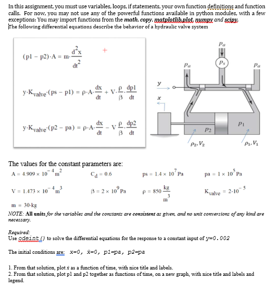
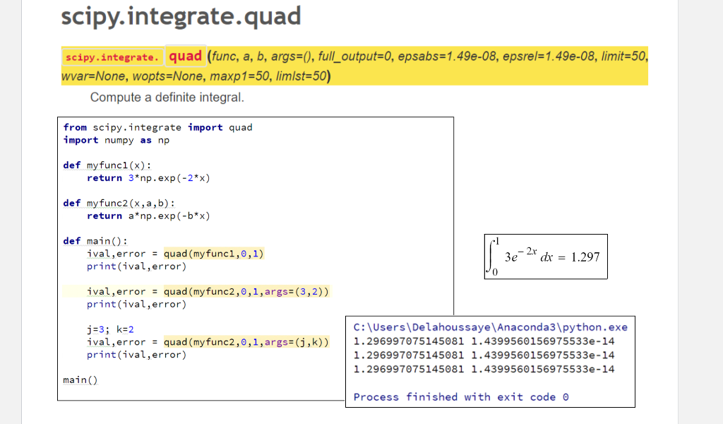
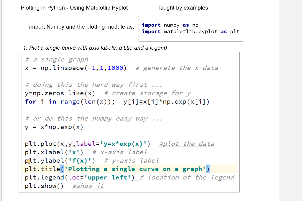
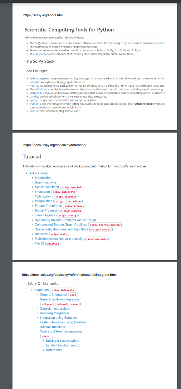
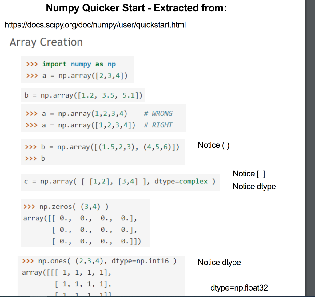
scipy.integrate.quad scipy.integrate. quad (func, a, b, args=(), full_output=0, epsabs=1.49e-08, epsrel=1.49e-08, limit=50, wvar=None, wopts=None, maxp1=50, limist=50) Compute a definite integral. from scipy.integrate import quad import numpy as np def my func1(x): return 3* np.exp(-2*x) def my func2(x, a,b): return a*np.exp(-b*x) -1 def main(): ival, error = quad(my func1,0,1) print(ival, error) 3e 2x dx = 1.297 ival, error = quad (my func2,0,1,args=(3,2)) print(ival, error) j=3; k=2 ival,error = quad (my func2,0,1, args=(j,k)) print(ival, error) C:\Users\Delahoussaye Anaconda3\python.exe 1.296997075145081 1.4399560156975533e-14 1.296997075145081 1.4399560156975533e-14 1.296997075145081 1.4399560156975533e-14 main Process finished with exit code o Plotting in Python - Using Matplotlib Pyplot Taught by examples: import Numpy and the plotting module as: import numpy as np import matplotlib.pyplot as plt 1. Plot a single curve with axis labels, a title and a legend # a single graph x = np.linspace(-1,1,1000) # generate the x-data # doing this the hard way first ... y=np.zeros_like (x) # create storage for y for i in range (len(x)); y[i]=x[i]*np.exp(x[i]) # or do this the numpy easy way ... y = x*np.exp(x) plt.plot(x,y,label='y=x*exp(x)') #plot the data plt.xlabel('x') # x-axis label plt.ylabel('f(x)') # y-axis label plt.title('Plotting a single curve on a graph') plt.legend (loc='upper left') # location of the legend plt.show() #show it https://scipy.org/about.html Scientific Computing Tools for Python Scipy refers to several related but distinct entities: The Scipy Stack, a collection of open source software for scientific computing in Python, and particularly a specified The community of people who use and develop this stack. . Several conferences dedicated to scientific computing in Python - Scipy, EuroScipy and Scipy.in. The Scipy library, one component of the SciPy stack, providing many numerical routines. The Scipy Stack Core Packages Python, a general purpose programming language. It is interpreted and dynamically typed and is very suited for int powerful enough to write large applications in NumPy, the fundamental package for numerical computation. It defines the numerical array and matrix types and The Scipy library, a collection of numerical algorithms and domain-specific toolboxes, including signal processing a Matplotlib, a mature and popular plotting package, that provides publication quality 2D plotting as well as rudimen pandas, providing high-performance, easy to use data structures. Sympy, for symbolic mathematics and computer algebra. IPython, a rich interactive interface, letting you quickly process data and test ideas. The IPython notebook works in computation in an easily reproducible form nose, a framework for testing Python code. https://docs.scipy.org/doc/scipy/reference/ Tutorial Tutorials with worked examples and background information for most Scipy submodules. SciPy Tutorial o Introduction Basic functions Special functions (scipy.special) Integration (scipy, integrate) Optimization (scipy optimize) Interpolation ( sipy. Interpolate) Fourier Transforms (scipy.fftpack ) Signal Processing scipy.signal) Linear Algebra scipy. linals Sparse Eigenvalue Problems with ARPACK Compressed Sparse Graph Routines (scipy,sparse.csgraph) Spatial data structures and algorithms scipy.spatial) Statistics (scipy.stats ) Multidimensional image processing scipy.ndimape) File 10 (scipy.io ) https://docs.scipy.org/doc/scipy/reference/tutorial/integrate.html Table of Contents Integration (scipy integrate) General integration (quad) General multiple integration (, dblquad, tplquadnquad ) Gaussian quadrature Romberg Integration Integrating using Samples Faster integration using low-level callback functions - Ordinary differential equations (odeint) Solving a system with a banded Jacobian matrix . References Numpy Quicker Start - Extracted from: https://docs.scipy.org/documpy/user/quickstart.html Array Creation >>> import numpy as np >>> a = np.array([2,3,4]) b = np.array([1.2, 3.5, 5.1]) >>> a = np.array(1,2,3,4) # WRONG np.array([1,2,3,4]) # RIGHT >>> a = >>> b = np.array([(1.5,2,3), (4,5,6)]) Notice () >>> b C = np.array( [[1,2], [3,4] ], dtype=complex ) Notice [ ] Notice dtype >>> np.zeros( (3,4) ) array([[ 0., 0., 0., 0.), [ 0., 0., 0., 0.], [ 0., 0., 0., 0.]]) Notice dtype >>> np.ones( (2,3,4), dtype=np. int16 ) array([[[ 1, 1, 1, 1], [ 1, 1, 1, 1], dtype=np.float32 111 In this assignment, you must use variables, loops, if statements, your own function definitions and function calls. For now, you may not use any of the powerful functions available in python modules, with a few exceptions: You may import functions from the math, copy, matrletlibrlot numpy and scirx. The following differential equations describe the behavior of a hydraulic valve system Pa (pl - p2) A = m- Pa Pa y-Kvalve (ps - pl) = p.4. dx + v.2 dpl dt B dt x PI dx y Kvalve (P2 - pa) = p.A. v L.dp2 dt P2 Bdt P2. Pi.V The values for the constant parameters are: A = 4.909 10- *m? Ca = 0.6 ps = 1.4 x 10 Pa pa = 1 x 10 Pa V = 1.473 x 10-43 3 = 2 x 10' Pa p = 850 kg Kvalve = 2-105 m = 30-kg NOTE: All units for the variables and the constants are consistent given, and no unit conversions of any kind are necessary Required: Use odeint/) to solve the differential equations for the response to a constant input of y=0.002 The initial conditions are: x=0, x=0, pi=pa, p2=pa 1. From that solution, plot x as a function of time, with nice title and labels. 2. From that solution, plot pl and p2 together as functions of time, on a new graph, with nice title and labels and legend. scipy.integrate.quad scipy.integrate. quad (func, a, b, args=(), full_output=0, epsabs=1.49e-08, epsrel=1.49e-08, limit=50, wvar=None, wopts=None, maxp1=50, limist=50) Compute a definite integral. from scipy.integrate import quad import numpy as np def my func1(x): return 3* np.exp(-2*x) def my func2(x, a,b): return a*np.exp(-b*x) -1 def main(): ival, error = quad(my func1,0,1) print(ival, error) 3e 2x dx = 1.297 ival, error = quad (my func2,0,1,args=(3,2)) print(ival, error) j=3; k=2 ival,error = quad (my func2,0,1, args=(j,k)) print(ival, error) C:\Users\Delahoussaye Anaconda3\python.exe 1.296997075145081 1.4399560156975533e-14 1.296997075145081 1.4399560156975533e-14 1.296997075145081 1.4399560156975533e-14 main Process finished with exit code o Plotting in Python - Using Matplotlib Pyplot Taught by examples: import Numpy and the plotting module as: import numpy as np import matplotlib.pyplot as plt 1. Plot a single curve with axis labels, a title and a legend # a single graph x = np.linspace(-1,1,1000) # generate the x-data # doing this the hard way first ... y=np.zeros_like (x) # create storage for y for i in range (len(x)); y[i]=x[i]*np.exp(x[i]) # or do this the numpy easy way ... y = x*np.exp(x) plt.plot(x,y,label='y=x*exp(x)') #plot the data plt.xlabel('x') # x-axis label plt.ylabel('f(x)') # y-axis label plt.title('Plotting a single curve on a graph') plt.legend (loc='upper left') # location of the legend plt.show() #show it https://scipy.org/about.html Scientific Computing Tools for Python Scipy refers to several related but distinct entities: The Scipy Stack, a collection of open source software for scientific computing in Python, and particularly a specified The community of people who use and develop this stack. . Several conferences dedicated to scientific computing in Python - Scipy, EuroScipy and Scipy.in. The Scipy library, one component of the SciPy stack, providing many numerical routines. The Scipy Stack Core Packages Python, a general purpose programming language. It is interpreted and dynamically typed and is very suited for int powerful enough to write large applications in NumPy, the fundamental package for numerical computation. It defines the numerical array and matrix types and The Scipy library, a collection of numerical algorithms and domain-specific toolboxes, including signal processing a Matplotlib, a mature and popular plotting package, that provides publication quality 2D plotting as well as rudimen pandas, providing high-performance, easy to use data structures. Sympy, for symbolic mathematics and computer algebra. IPython, a rich interactive interface, letting you quickly process data and test ideas. The IPython notebook works in computation in an easily reproducible form nose, a framework for testing Python code. https://docs.scipy.org/doc/scipy/reference/ Tutorial Tutorials with worked examples and background information for most Scipy submodules. SciPy Tutorial o Introduction Basic functions Special functions (scipy.special) Integration (scipy, integrate) Optimization (scipy optimize) Interpolation ( sipy. Interpolate) Fourier Transforms (scipy.fftpack ) Signal Processing scipy.signal) Linear Algebra scipy. linals Sparse Eigenvalue Problems with ARPACK Compressed Sparse Graph Routines (scipy,sparse.csgraph) Spatial data structures and algorithms scipy.spatial) Statistics (scipy.stats ) Multidimensional image processing scipy.ndimape) File 10 (scipy.io ) https://docs.scipy.org/doc/scipy/reference/tutorial/integrate.html Table of Contents Integration (scipy integrate) General integration (quad) General multiple integration (, dblquad, tplquadnquad ) Gaussian quadrature Romberg Integration Integrating using Samples Faster integration using low-level callback functions - Ordinary differential equations (odeint) Solving a system with a banded Jacobian matrix . References Numpy Quicker Start - Extracted from: https://docs.scipy.org/documpy/user/quickstart.html Array Creation >>> import numpy as np >>> a = np.array([2,3,4]) b = np.array([1.2, 3.5, 5.1]) >>> a = np.array(1,2,3,4) # WRONG np.array([1,2,3,4]) # RIGHT >>> a = >>> b = np.array([(1.5,2,3), (4,5,6)]) Notice () >>> b C = np.array( [[1,2], [3,4] ], dtype=complex ) Notice [ ] Notice dtype >>> np.zeros( (3,4) ) array([[ 0., 0., 0., 0.), [ 0., 0., 0., 0.], [ 0., 0., 0., 0.]]) Notice dtype >>> np.ones( (2,3,4), dtype=np. int16 ) array([[[ 1, 1, 1, 1], [ 1, 1, 1, 1], dtype=np.float32 111 In this assignment, you must use variables, loops, if statements, your own function definitions and function calls. For now, you may not use any of the powerful functions available in python modules, with a few exceptions: You may import functions from the math, copy, matrletlibrlot numpy and scirx. The following differential equations describe the behavior of a hydraulic valve system Pa (pl - p2) A = m- Pa Pa y-Kvalve (ps - pl) = p.4. dx + v.2 dpl dt B dt x PI dx y Kvalve (P2 - pa) = p.A. v L.dp2 dt P2 Bdt P2. Pi.V The values for the constant parameters are: A = 4.909 10- *m? Ca = 0.6 ps = 1.4 x 10 Pa pa = 1 x 10 Pa V = 1.473 x 10-43 3 = 2 x 10' Pa p = 850 kg Kvalve = 2-105 m = 30-kg NOTE: All units for the variables and the constants are consistent given, and no unit conversions of any kind are necessary Required: Use odeint/) to solve the differential equations for the response to a constant input of y=0.002 The initial conditions are: x=0, x=0, pi=pa, p2=pa 1. From that solution, plot x as a function of time, with nice title and labels. 2. From that solution, plot pl and p2 together as functions of time, on a new graph, with nice title and labels and legend