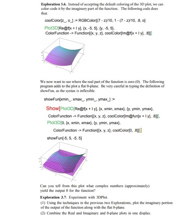
Exploration 3.6. Instead of accepting the default coloring of the 3D plot, we can color-code it by the imaginary part of the function. The following code does that. coolColor[z_, 0_]:= RGB Colorf(7-2)/10, 1-(7 - Zy10,-8, 0] Plot3D(Re@f[x + 1 y). {X-5, 5}, {y. -5,5), ColorFunction -> Function[{x, y, z, coolColorfm@f(x + y), .8]]] We now want to see where the real part of the function is zero (O). The following program adds to the plot a flat 0-plane. Be very careful in typing the definition of showFun, as the syntax is inflexible. showFun[xmin_, xmax_, ymin_, ymax_] := Show[Plot3D [Re@flx + y). {x, xmin, xmax}, {y, ymin, ymax}. ColorFunction -> Function[{x, y, z), coolColor[Im@fun[x + ly]..8]]. Plot3D(0, {x, xmin, xmax}, {y, ymin, ymax). ColorFunction -> Function[{x, y, z), coolColor(0, 8]]] showFun(-5, 5, -5,5) Can you tell from this plot what complex numbers (approximately) yield the output 0 for the function? Exploration 3.7: Experiment with 3DPlot. (1) Using the techniques in the previous two Explorations, plot the imaginary portion of the output of the function along with the flat O-plane. (2) Combine the Real and Imaginary and O-plane plots in one display. Exploration 3.6. Instead of accepting the default coloring of the 3D plot, we can color-code it by the imaginary part of the function. The following code does that. coolColor[z_, 0_]:= RGB Colorf(7-2)/10, 1-(7 - Zy10,-8, 0] Plot3D(Re@f[x + 1 y). {X-5, 5}, {y. -5,5), ColorFunction -> Function[{x, y, z, coolColorfm@f(x + y), .8]]] We now want to see where the real part of the function is zero (O). The following program adds to the plot a flat 0-plane. Be very careful in typing the definition of showFun, as the syntax is inflexible. showFun[xmin_, xmax_, ymin_, ymax_] := Show[Plot3D [Re@flx + y). {x, xmin, xmax}, {y, ymin, ymax}. ColorFunction -> Function[{x, y, z), coolColor[Im@fun[x + ly]..8]]. Plot3D(0, {x, xmin, xmax}, {y, ymin, ymax). ColorFunction -> Function[{x, y, z), coolColor(0, 8]]] showFun(-5, 5, -5,5) Can you tell from this plot what complex numbers (approximately) yield the output 0 for the function? Exploration 3.7: Experiment with 3DPlot. (1) Using the techniques in the previous two Explorations, plot the imaginary portion of the output of the function along with the flat O-plane. (2) Combine the Real and Imaginary and O-plane plots in one display