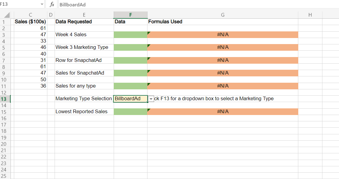
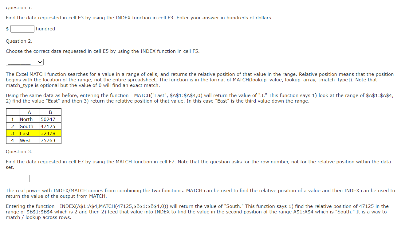
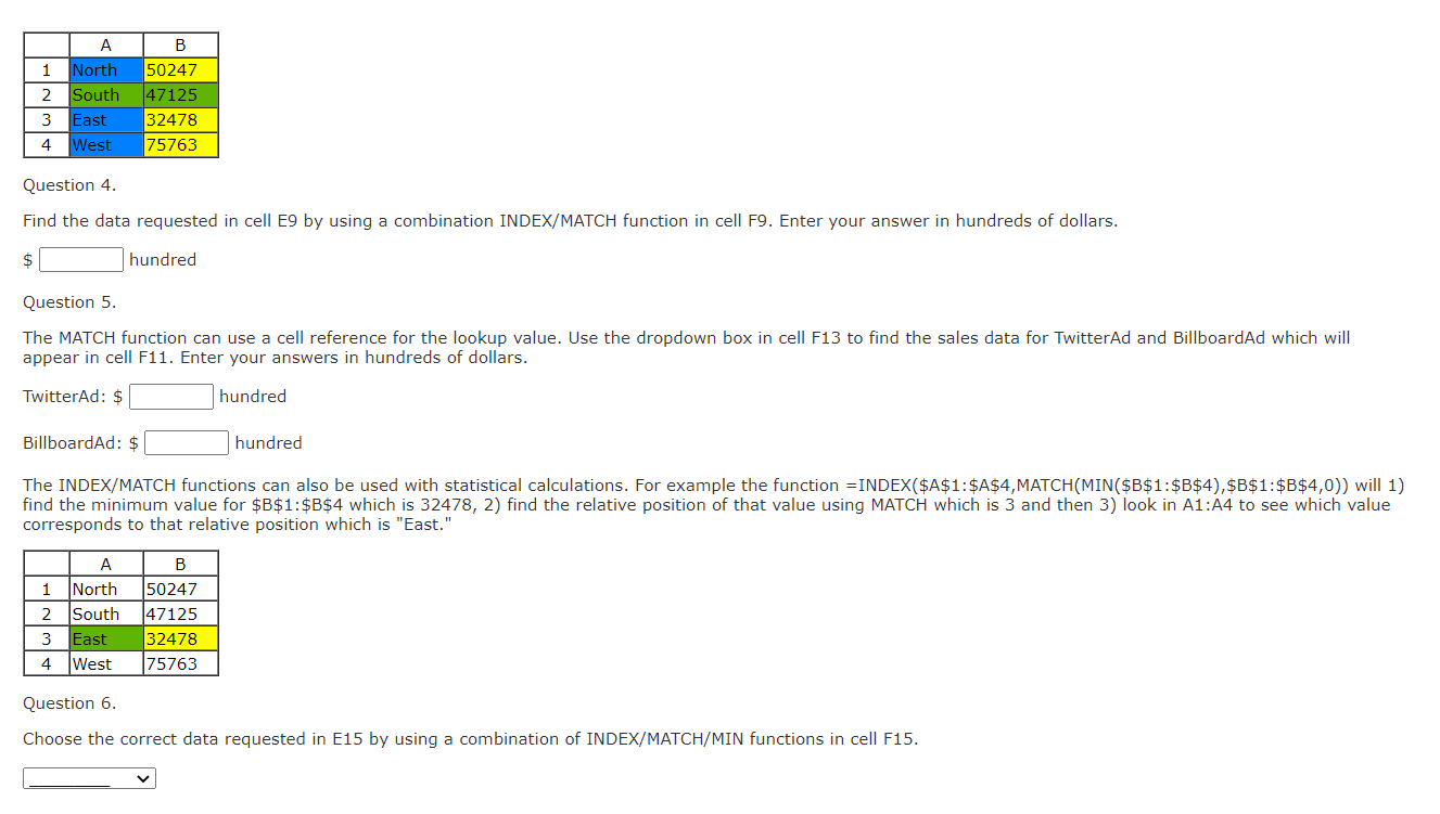
F13 fx Billboard Ad G H E Data Requested Data Formulas Used Week 4 Sales #N/A Week 3 Marketing Type #N/A Sales ($100s) 61 47 33 46 40 31 61 47 50 36 Row for SnapchatAd #N/A Sales for SnapchatAd #N/A Sales for any type #N/A 1 2 3 4 5 6 7 8 9 10 11 12 13 14 15 16 17 18 19 20 21 22 23 24 25 Marketing Type Selection Billboard Ad ck F13 for a dropdown box to select a Marketing Type Lowest Reported Sales #N/A Question 1. Find the data requested in cell E3 by using the INDEX function in cell F3. Enter your answer in hundreds of dollars. $ hundred Question 2. Choose the correct data requested in cell E5 by using the INDEX function in cell F5. The Excel MATCH function searches for a value in a range of cells, and returns the relative position of that value in the range. Relative position means that the position begins with the location of the range, not the entire spreadsheet. The function is in the format of MATCH(lookup_value, lookup_array, [match_type]). Note that match_type is optional but the value of 0 will find an exact match. Using the same data as before, entering the function =MATCH("East", $A$1:$A$4,0) will return the value of "3." This function says 1) look at the range of $A$1:$A$4, 2) find the value "East" and then 3) return the relative position of that value. In this case "East" is the third value down the range. B 1 2 3 4 . North South East West 50247 47125 32478 75763 Question 3. Find the data requested in cell E7 by using the MATCH function in cell F7. Note that the question asks for the row number, not for the relative position within the data set. The real power with INDEX/MATCH comes from combining the two functions. MATCH can be used to find the relative position of a value and then INDEX can be used to return the value of the output from MATCH. Entering the function =INDEX(A$1:A$4, MATCH(47125,$B$1:$B$4,0)) will return the value of "South." This function says 1) find the relative position of 47125 in the range of $B$1:$B$4 which is 2 and then 2) feed that value into INDEX to find the value in the second position of the range A$1:A$4 which is "South." It is a way to match / lookup across rows. |||| North South East West B 50247 47125 32478 75763 3 4 Question 4. Find the data requested in cell E9 by using a combination INDEX/MATCH function in cell F9. Enter your answer in hundreds of dollars. $ hundred Question 5. The MATCH function can use a cell reference for the lookup value. Use the dropdown box in cell F13 to find the sales data for TwitterAd and BillboardAd which will appear in cell F11. Enter your answers in hundreds of dollars. TwitterAd: $ hundred BillboardAd: $ hundred The INDEX/MATCH functions can also be used with statistical calculations. For example the function =INDEX($A$1:$A$4,MATCH(MIN($B$1:$B$4),$B$1:$B$4,0)) will 1) find the minimum value for $B$1:$B$4 which is 32478, 2) find the relative position of that value using MATCH which is 3 and then 3) look in A1:A4 to see which value corresponds to that relative position which is "East." B 1 North 2 South 3 East 4 West 50247 47125 32478 75763 Question 6. Choose the correct data requested in E15 by using a combination of INDEX/MATCH/MIN functions in cell F15. F13 fx Billboard Ad G H E Data Requested Data Formulas Used Week 4 Sales #N/A Week 3 Marketing Type #N/A Sales ($100s) 61 47 33 46 40 31 61 47 50 36 Row for SnapchatAd #N/A Sales for SnapchatAd #N/A Sales for any type #N/A 1 2 3 4 5 6 7 8 9 10 11 12 13 14 15 16 17 18 19 20 21 22 23 24 25 Marketing Type Selection Billboard Ad ck F13 for a dropdown box to select a Marketing Type Lowest Reported Sales #N/A Question 1. Find the data requested in cell E3 by using the INDEX function in cell F3. Enter your answer in hundreds of dollars. $ hundred Question 2. Choose the correct data requested in cell E5 by using the INDEX function in cell F5. The Excel MATCH function searches for a value in a range of cells, and returns the relative position of that value in the range. Relative position means that the position begins with the location of the range, not the entire spreadsheet. The function is in the format of MATCH(lookup_value, lookup_array, [match_type]). Note that match_type is optional but the value of 0 will find an exact match. Using the same data as before, entering the function =MATCH("East", $A$1:$A$4,0) will return the value of "3." This function says 1) look at the range of $A$1:$A$4, 2) find the value "East" and then 3) return the relative position of that value. In this case "East" is the third value down the range. B 1 2 3 4 . North South East West 50247 47125 32478 75763 Question 3. Find the data requested in cell E7 by using the MATCH function in cell F7. Note that the question asks for the row number, not for the relative position within the data set. The real power with INDEX/MATCH comes from combining the two functions. MATCH can be used to find the relative position of a value and then INDEX can be used to return the value of the output from MATCH. Entering the function =INDEX(A$1:A$4, MATCH(47125,$B$1:$B$4,0)) will return the value of "South." This function says 1) find the relative position of 47125 in the range of $B$1:$B$4 which is 2 and then 2) feed that value into INDEX to find the value in the second position of the range A$1:A$4 which is "South." It is a way to match / lookup across rows. |||| North South East West B 50247 47125 32478 75763 3 4 Question 4. Find the data requested in cell E9 by using a combination INDEX/MATCH function in cell F9. Enter your answer in hundreds of dollars. $ hundred Question 5. The MATCH function can use a cell reference for the lookup value. Use the dropdown box in cell F13 to find the sales data for TwitterAd and BillboardAd which will appear in cell F11. Enter your answers in hundreds of dollars. TwitterAd: $ hundred BillboardAd: $ hundred The INDEX/MATCH functions can also be used with statistical calculations. For example the function =INDEX($A$1:$A$4,MATCH(MIN($B$1:$B$4),$B$1:$B$4,0)) will 1) find the minimum value for $B$1:$B$4 which is 32478, 2) find the relative position of that value using MATCH which is 3 and then 3) look in A1:A4 to see which value corresponds to that relative position which is "East." B 1 North 2 South 3 East 4 West 50247 47125 32478 75763 Question 6. Choose the correct data requested in E15 by using a combination of INDEX/MATCH/MIN functions in cell F15