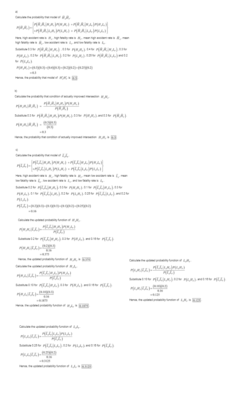
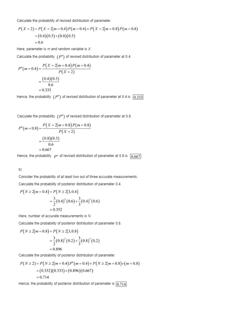
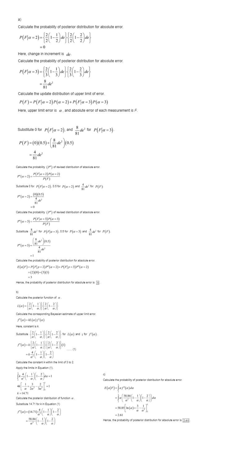
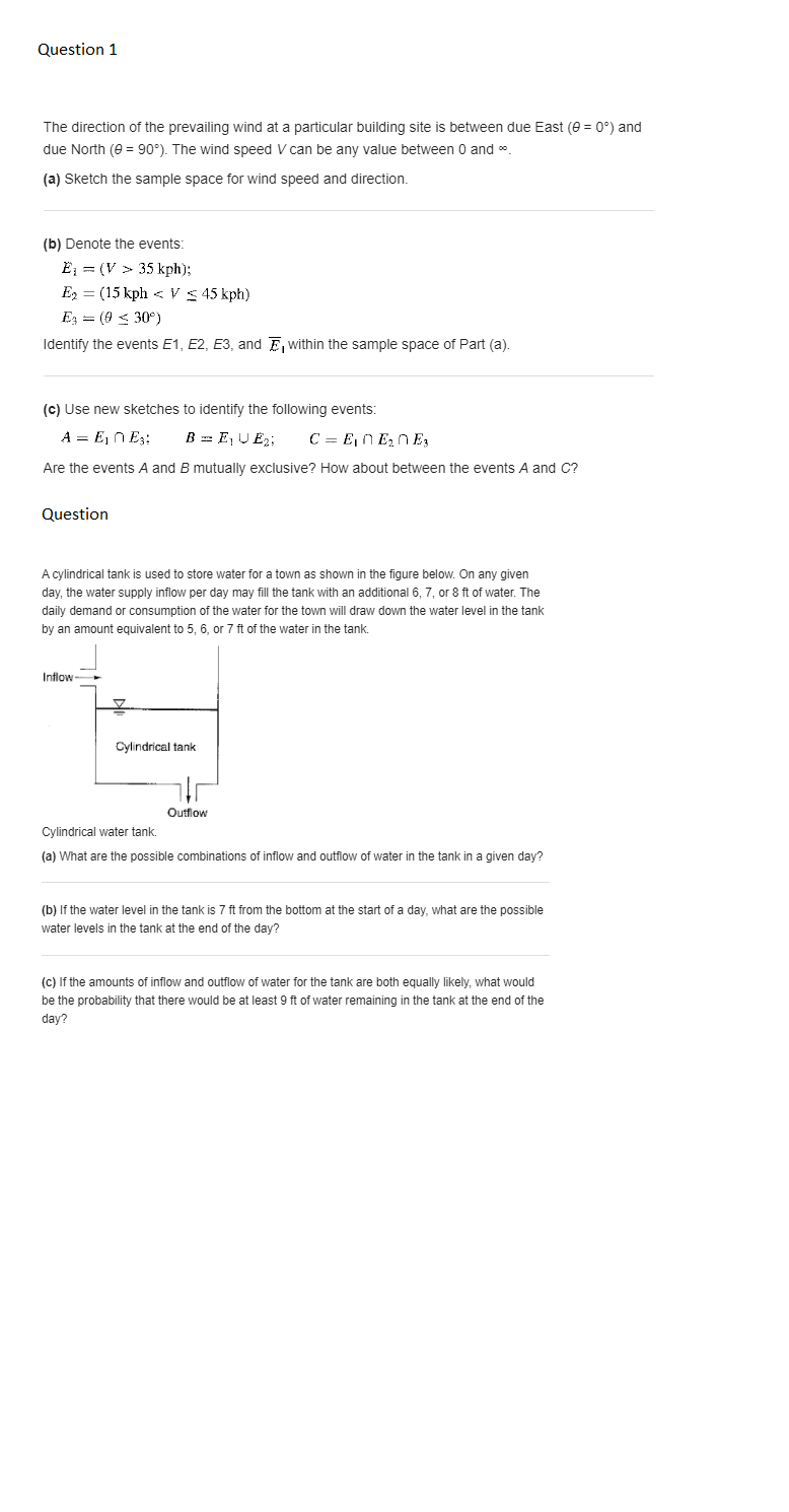
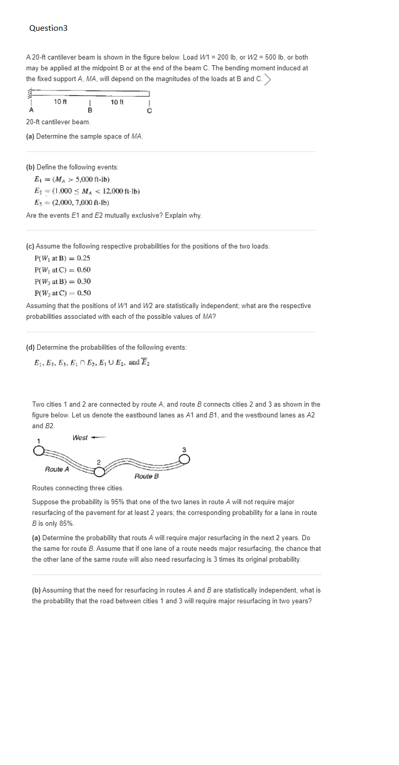
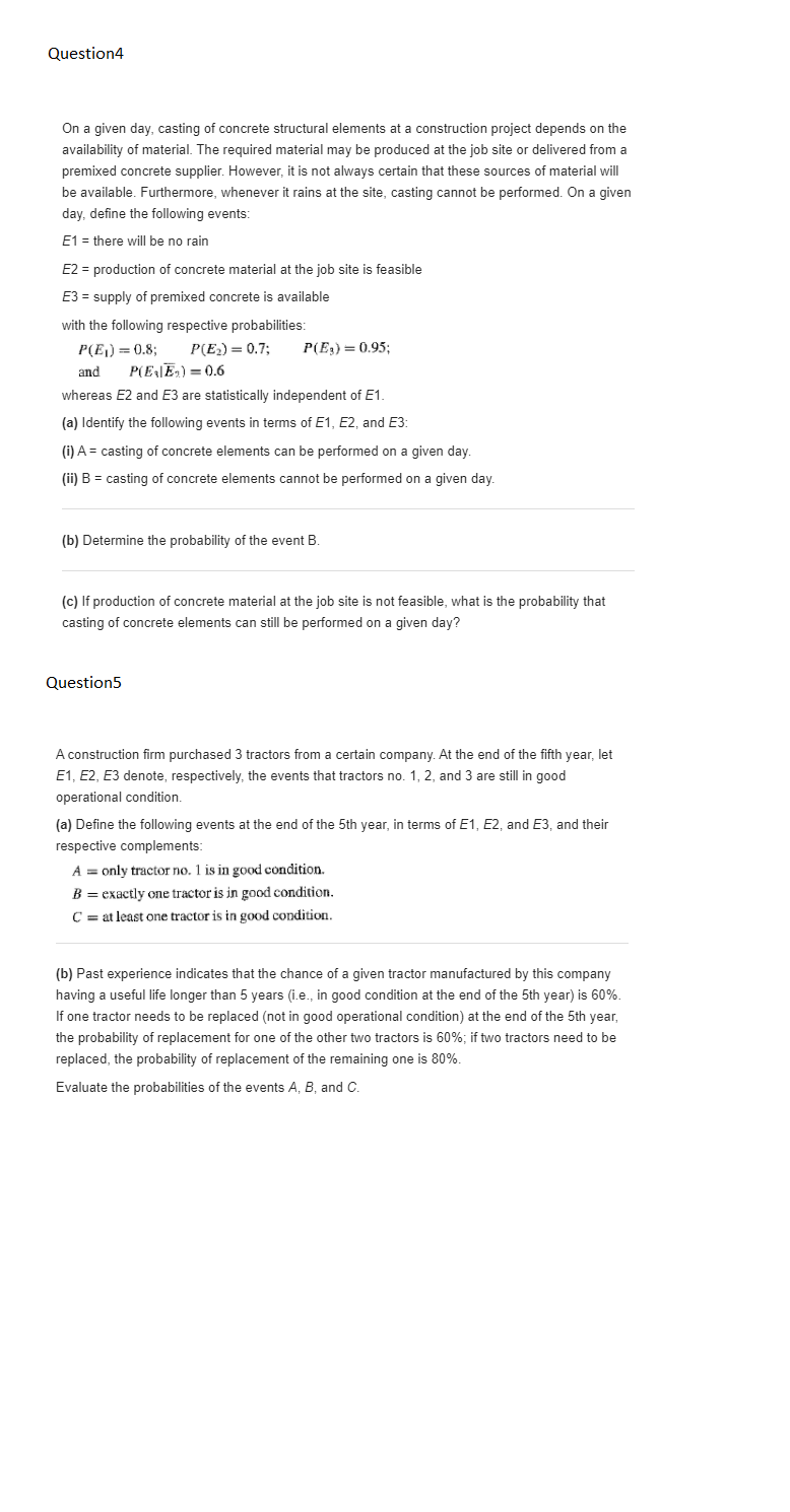
\f\f\f\f\f\fCalculate the expected probability (p) of survival before proof test. Consider the probability structure survive the maximum load of 0.90 which reliable at 70%. However, the probability of 0.50 reliable at 25% and the probability of 0.10 may be 5% P(S|p= 0.90) P(p = 0.90) +P(S|p=0.50) P(p = 0.50) +P(S|p=0.10) P(P=0.10) Here, survival of probability structure is P(S). Substitute 0.90 for P(S| p = 0.90). 0.70 for P(p = 0.90), 0.50 for P(S|p = 0.50). 0.25 for P(p =0.50), 0.10 for P(S| p = 0.10) and 0.05 for P(p= 0.10). p =(0.90)(0.70) +(0.50)(0.25) +(0.10)(0.05) = 0.76 Hence, the expected probability (p) of survival before proof test is 10.761. b) Calculate the distribution (P") of survival probability at proof load of 0.90. Consider that one structure is tested and survive at maximum proof load P"(p= 0.90) = ( Elp = 0.90) P(p = 0.90) P(E) Here, one probability structure survive the proof test is P(E). Substitute 0.76 for P(E), 0.90 for P(E|p= 0.90) and 0.70 for P(p = 0.90) P'(p=0.90) = (0.90) (0.70) 0.76 : 0.83 Hence, the distribution (P") of survival probability at proof load of 0.90 is 0.83]. Calculate the distribution (P") of survival probability at proof load of 0.50. Consider that one structure is tested and survive at maximum proof load. P"(p=0.50) = ( Elp = 0.50) P(p = 0.50) P(E) Here, one probability structure survive the proof test is P(E) Substitute 0.76 for P(E). 0.50 for P(Elp = 0.50) and 0.25 for P(p = 0.50) P' (p=0.50) = (0.50) (0.25) 0.76 =0.16 Hence, the distribution (P") of survival probability at proof load of 0.50 is [0.16]. Calculate the distribution (P") of survival probability at proof load of 0.10. Consider that one structure is tested and survive at maximum proof load. P' (p= 0.10) = P(E p = 0.10) P(p = 0.10) P(E) Here, one probability structure survive the proof test is P(E) Substitute 0.76 for P(E), 0.10 for P( E|p =0.10) and 0.05 for P(p = 0.10) P" (p = 0.10) = (0.10)(0.05) 0.76 = 0.01 Hence, the distribution (P") of survival probability at proof load of 0.10 is [0.01] c) Calculate the update expected probability of survival. P(p=0.9/E)= EP.P"(P=P.) [P(Elp=0.90) P" (p=0.90)+ P(E|p =0.50) P" (p=0.50)1 +P(E| p =0.10) P'(p = 0.10) Substitute 0.90 for P(E| p = 0.90), 0.83 for P"(p= 0.90). 0.50 for P(E| p = 0.50), 0.16 for P"(p=0.50), 0.10 for P(Elp= 0.10) and 0.01 for P"(p= 0.10). P(P=0.9|E)=(0.90)(0.83)+(0.50)(0.16)+(0.10)(0.01) =0.828 Hence the update expected probability of survival is 0.828 d) Calculate the proof. JP(AP=0.90) P(p =0.90)+P(4p=0.50)P(p=0.50) +P(4p=0.10) P(p =0.10) )(09) (0.10)(0.70)+=(050)'(0.50 )(0.25) -(0.10)'(0.90)(0.05) -0.17+0.0937 +0.0013 -0.265 Calculate the expected probability of survival at proof load of 0.90. P(P-0.90)4)_ ( 4p-0.90) P(p -0.90) P(A) (0.9)'(0.10)(0.70) P(4) Substitute 0.265 for P(4) P(P=0.90)4)- 2 (0.9) (0.10)(0.70) 0.265 0.17 0 265 - 0.64 Calculate the expected probability of survival at proof load of 0. 10. Calculate the expected probability of survival at proof load of 0.50. P(P-0.10|4) _ (4p-0.10)P(p =0.10) P(P=0.50|4) _ (4p - 0.50) P(p= 0.50) P(A) P(4) (0.10)'(0.90)(0.05) (0.50)' (0.50)(0.25) P (A) P(A) Substitute 0.265 for P(4). Substitute 0.265 for P(A) 2(0.10)' (0.90)(0.05) P(P =0.50 4) - 2 (0.50)' (0.50)(0.25) P(P-0.10)4) - 2 0.265 0.265 0.0013 0.265 0.265 -0.01 -0.35 Calculate the update expected probability of survival. E(PA)= P(El p =0.90) P(P= 0.90)4)+P(E\\ p =0.50) P(P= 0.50|4) +P(E| p =0.10) P(P =0.10|4) Substitute 0.90 for P(Elp = 0.90). 0.64 for P(P= 0.90|4). 0.50 for P( Elp = 0.50). 0.35 for P(P=0.50|4). 0.10 for P(Elp = 0.10) and 0.01 for P(P=0.10|4). E(P| 4) - (0.90)(0.64)+(0.50)(0.35)+(0.10)(0.01) = 0.752 ence. the update expected probability of survival is [0.752].a) Calculate the probability that model of H,H, P( R, A.)= P(A,A, [H.H.) P(H, H.) + P(A, A,[H,L, ) P(H,L.) +P(R, A.[L, H,) P(L, H.) + P(R, A.|LL, ) P(L,L, )] Here. high accident rate is A, , high fatality rate is My, mean high accident rate is #,. mean high fatality rate is /, . low accident rate is L, , and low fatality rate is Ly. Substitute 0.3 for P(H, H.( H, H.) . 0.3 for P( H, H.). 0.4 for P( H, H.[ H, L. ). 0.3 for P(H, L,). 0.2 for P( H, H.(L, H.). 0.2 for P(L, H, ). 0.25 for P( H, H,( L, L, ) and 0.2 for P( L,L,). P(H, H,) = (0.3)(0.3)+(0.4)(0.3)+(0.2)(0.2)+(0.25)(0.2) =0.3 Hence, the probability that model of I'M; is [0 3]. Calculate the probability that condition of actually improved intersection H,H, P(H. H,|A,H.) - P( H H,| H , H. )P(H, H.) P(H, H,) Substitute 0.3 for P( H, H,[ H, H, ) P( H, H.). 0.3 for P(H, H, ). and 0.3 for P( R, H.)- P(H, H.[A,A,) _ (0.3)(0.3) (0.3) =0.3 Hence, the probability that condition of actually improved intersection N,#, is [0 3]. c) Calculate the probability that model of L, L,- P ( I, [, ) = JP(I, [, [ H, H. ) P(H, H.) + P(I,[, [ H,L. ) P(H,L, ) +P([, [,| L. H, ) P(L, H. ) + P(I, I,|L.L. ) P(L,4. ) ] Here. high accident rate is /, . high fatality rate is #,. mean low accident rate is [,. mean low fatality rate is Zy . low accident rate is Ly . and low fatality rate is Ly- Substitute 0.2 for P(L,L,[ H, H. ). 0.3 for P( H, H. ). 0.1 for P(I, [,( H, L, ). 0.3 for P(H, L, ). 0.1 for P([,[,| L, H. ). 0.2 for P( L, H, ). 0.25 for P( I, [ ( L, L, ). and 0.2 for P (L, L, ) P(I,I,)-(0.2)(0.3)+(0.1)(0.3) +(0.1)(0.2)+(0.25)(0.2) =0.16 Calculate the updated probability function of H,H,. P( H, H. | Z,I, ) _ P( L. L. H, H. ) P( H,L, ) P(L,Z, ) Substitute 0.2 for P([, L,( H, H, ). 0.3 for P( H, L, ). and 0.16 for P(L,L.) P(H, H.[[,I, )_ (0.2)(0.3) 0.16 = 0.375 Hence, the updated probability function of H,M, is [0.375]- Calculate the updated probability function of L, H, Calculate the updated probability function of H ,Ly. P(L, H,|[,I, )_ ( LL, L, H. ) P ( L, H, ) P( H, L, | LL,) - - P(L, L, H ,L, ) P( H , L.) P(L, Ly) P(LL,) Substitute 0.10 for P([,[,| L, H. ). 0.2 for P(L, H, ). and 0.16 for P(I,L. ) Substitute 0.10 for P(L, L,( H, L, ). 0.3 for P(H, Ly ). and 0.16 for P(L, Ly ). P(L, H,[[,[, )_ (0.10)(0.2) P(H,L.[[,I, )- (0.10)(0.3) 0.16 0.16 =0.125 =0.1875 Hence, the updated probability function of 1,H, is [0.125] Hence, the updated probability function of H,, is [0. 1875] Calculate the updated probability function of L,1- P ( L L,[I,I, ) _ (LL LL, ) P (L, L, ) P(LL, ) Substitute 0.25 for P(I, L.| L, L, ). 0.2 for P(L, L, ). and 0.16 for P(C,[. ). P(L,L,[[,[, ) (0.25)(0.2) 0.16 =0.3125 Hence, the updated probability function of L L, is 0.3125]-Calculate the probability of revised distribution of parameter. P(X = 2) = P(X = 2|m = 0.4) P(m = 0.4)+ P(X = 2\\m = 0.8) P(m = 0.8) = (0.4)(0.5)+(0.8)(0.5) =0.6 Here, parameter is m and random variable is X. Calculate the probability (p* ) of revised distribution of parameter at 0.4. P' (m = 0.4) = P(X = 2)m = 0.4) P(m = 0.4) P(X = 2) (0.4) (0.5) 0.6 = 0.333 Hence, the probability (P") of revised distribution of parameter at 0.4 is 0.333 Calculate the probability (P") of revised distribution of parameter at 0.8. P(m =0.8) = P(X = 2|m = 0.8) P(m = 0.8) P(X =2) (0.8) (0.5) 0.6 =0.667 Hence, the probability p* of revised distribution of parameter at 0.8 is 0.667 b) Consider the probability of at least two out of three accurate measurements. Calculate the probability of posterior distribution of parameter 0.4. P(N 2 2)m = 0.4) = P(N 2 2|3,0.4) -(0.4) (0.6)+2(0.4)'(0.6) = 0.352 Here, number of accurate measurements is N. Calculate the probability of posterior distribution of parameter 0.8. P(N 2 2)m = 0.8) = P(N 2 2|3, 0.8) (0.8)'(0.2)+ =(0.8)'(0.2) =0.896 Calculate the probability of posterior distribution of parameter. P(N 2 2) = P(N 2 2\\m =0.4) P"(m = 0.4)+P(N 2 2|m = 0.8)v(m = 0.8) = (0.352)(0.333)+(0.896)(0.667) =0.714 Hence, the probability of posterior distribution of parameter is [0.714-a) Calculate the probability of posterior distribution for absolute error. P( Fla = 2)= (1-; ) de} 2(1-2) de} =0 Here, change in increment is de. Calculate the probability of posterior distribution for absolute error. P(Fla = 3)= (1-;) de 3(1-3) de 8 81 Calculate the update distribution of upper limit of error. P(F) = P(Fla =2) P(a = 2)+P(Fla =3) P(a =3) Here, upper limit error is a , and absolute error of each measurement is F. Substitute 0 for P(Fla = 2), and del for P( Fla = 3) P(F)= (0)(0.5) +3 de (0.5) 81 -del Calculate the probability (P") of revised distribution of absolute error. P(a=2)= (Fla -2)P(a - 2) P(F) Substitute 0 for P(Fla = 2). 0.5 for P(a = 2) and - del for P(F)- P'(a =2) - 0)(0.5) Calculate the probability (P") of revised distribution of absolute error. P(a = 3) =4 P(Fa - 3) P(a - 3) P(F Substitute - de' for P( Fla =3). 0.5 for P(a =3) and - de' for P(F)- P(a = 3)= (81 de (0.5) Calculate the probability of posterior distribution for absolute error. E(a( F) = P(F(p=2) P' (a=2)+P(F\\p=3)P'(a=2) = (2)(0)+(3)(1) =3 Hence, the probability of posterior distribution for absolute error is [3]. b) Calculate the posterior function of a . Calculate the corresponding Bayesian estimate of upper limit error. f(a)=(a)f(a) Here. constant is k. Substitute 21-1 2(1 2 |for L(a ) and 1 for S'(a). "(a)-1 2(1-1 2(1-2) (1) ..... (1) -4 4(1-4( 1-4) Calculate the constant k within the limit of 3 to 2. Apply the limits in Equation (1) 1+41-4 1-2da =1 c) Calculate the probability of posterior distribution for absolute error. 44 1. 3 2 -1 La za 3 E(a F)=jaf(a)da A =14.71 Calculate the posterior distribution of function a . -Ja $8.84(1-1 1-2 Substitute 14.71 for k in Equation (1) -58.85 In(a)+3-4 "(a)=(14.71)4 (1-4(1-2) =2.61 _ 58.84 ( 1-1 1-2 Hence, the probability of posterior distribution for absolute error is [2.61]Question 1 The direction of the prevailing wind at a particular building site is between due East (0 = 0) and due North (0 = 90"). The wind speed V can be any value between 0 and co. (a) Sketch the sample space for wind speed and direction. (b) Denote the events: E1 = (V > 35 kph); E2 = (15 kph 10 ft 10 f 20-ft cantilever beam. (a) Determine the sample space of MA. (b) Define the following events: EI = (MA > 5,000 ft-1b) E2 = (1,000