file: simulate_python2.py

from mpl_toolkits.mplot3d import Axes3D

import matplotlib.pyplot as plt

import numpy as np

import random

import sys

def plot_gaussian(x,y,z,filename=None):

"""

Plot the multivariate Gaussian

If filename is not given, then the figure is not saved.

"""

# Note: there was no need to make this into a separate function

# however, it lets you see how to define functions within the

# main file, and makes it easier to comment out plotting if

# you want to experiment with many parameter changes without

# generating many, many graphs

fig = plt.figure()

ax = fig.add_subplot(111, projection='3d')

ax.scatter(x,y,z, c="red",marker="s")

ax.set_xlabel("X")

ax.set_ylabel("Y")

ax.set_zlabel("Z")

minlim, maxlim = -3, 3

ax.set_xlim(minlim,maxlim)

ax.set_ylim(minlim,maxlim)

ax.set_zlim(minlim,maxlim)

if filename is not None:

fig.savefig("scatter" + str(dim) + "_n" + str(numsamples) + ".png")

plt.show()

if __name__ == '__main__':

# default

dim = 1

numsamples = 100

if len(sys.argv) > 1:

dim = int(sys.argv[1])

if dim > 3:

print "Dimension must be 3 or less; capping at 3"

if len(sys.argv) > 2:

numsamples = int(sys.argv[2])

print "Running with dim = " + str(dim), \

" and numsamples = " + str(numsamples)

# Generate data from (multivariate) Gaussian

if dim == 1:

# mean and standard deviation in one dimension

mu = 0

sigma = 10

x = np.random.normal(mu, sigma, numsamples)

y = np.zeros(numsamples,)

z = np.zeros(numsamples,)

elif dim == 2:

# mean and standard deviation in two dimension

mu = [0,0]

sigma = [[1,0],[0,1]]

x,y = np.random.multivariate_normal(mu, sigma, numsamples).T

z = np.zeros(numsamples,)

else:

# mean and standard deviation in three dimension

mu = [0,0,0]

sigma = [[1,0,0],[0,1,0],[0,0,1]]

x,y,z = np.random.multivariate_normal(mu, sigma, numsamples).T

# Get the current estimate of the mean

print np.mean(x)

# Print all in 3d space, but just project to 2d or 1d

#plot_gaussian(x,y,z,"scatter" + str(dim) + "_n" + str(numsamples) + ".png")

plot_gaussian(x,y,z)

file: ass1ex.tex

\documentclass[11pt]{article} \usepackage{fancyheadings,multicol} \usepackage{amsmath,amssymb}

\setlength{\textheight}{\paperheight} \addtolength{\textheight}{-2in} \setlength{\topmargin}{-.5in} \setlength{\headsep}{.5in} \addtolength{\headsep}{-\headheight} \setlength{\footskip}{.5in} \setlength{\textwidth}{\paperwidth} \addtolength{\textwidth}{-2in} \setlength{\oddsidemargin}{0in} \setlength{\evensidemargin}{0in} \flushbottom

\allowdisplaybreaks

\pagestyle{fancyplain} \let\headrule=\empty \let\footrule=\empty \lhead{\fancyplain{}{Spring 2017}} head{\fancyplain{}{CSCI-B455: Machine Learning}} \cfoot{{\thepage/\pageref{EndOfAssignment}}}

ewcounter{totalmarks} \setcounter{totalmarks}{0} ewcounter{questionnumber} \setcounter{questionnumber}{0} ewcounter{subquestionnumber}[questionnumber] \setcounter{subquestionnumber}{0} enewcommand{\thesubquestionnumber}{(\alph{subquestionnumber})} ewcommand{\question}[2][]% {\ifx\empty#2\empty\else \addtocounter{totalmarks}{#2} efstepcounter{questionnumber}\fi \bigskip oindent\textbf{\Large Question \thequestionnumber. } #1 {\scshape\ifx\empty#2\empty(continued)\else [#2 mark\ifnum #2 > 1 s\fi]\fi}\par \medskip oindent\ignorespaces} ewcommand{\subquestion}[2][]% {\ifx\empty#2\empty\else efstepcounter{subquestionnumber}\fi \medskip oindent\textbf{\large \thesubquestionnumber } #1 {\scshape\ifx\empty#2\empty(continued)\else [#2 mark\ifnum #2 > 1 s\fi]\fi} \smallskip oindent\ignorespaces} ewcommand{\bonus}[2][]% {\bigskip oindent\textbf{\Large Bonus. } #1 {\scshape\ifx\empty#2\empty(continued)\else [#2 mark\ifnum #2 > 1 s\fi]\fi}\par \medskip oindent\ignorespaces}

\usepackage{totcount} egtotcounter{totalmarks}

\begin{document}

\thispagestyle{plain}

\begin{center} \bfseries {\Large Homework Assignment \# 1}\\ Due: Wednesday, February 1, 2017, 11:59 p.m. \\ Total marks: \total{totalmarks} \end{center}

\question{10}

Let $\Omega_X=\{a,b,c\}$ and $p_X(a)=0.1, p_X(b)=0.2$, and $p_X(c)=0.7$. Let % \begin{align*} f(x)= \left\{ \begin{array}{lr} 10 & \text{if } x = a\\ 5 & \text{if } x = b\\ 10/7 & \text{if } x = c \end{array} ight. \end{align*}

\subquestion{3} What is $E[f(x)]$?

\subquestion{3} What is $E[1/p_X(x)]$?

\subquestion{4} For an arbitrary pmf $p_X(x)$, what is $E[1/p_X(x)]$?

% You can also define new variables to make it easier % and avoid long commands ewcommand{\muvec}{\boldsymbol{\mu}}

\question{15} Let $\mathbf{X}_1, \ldots, \mathbf{X}_m$ be independent multivariate Gaussian random variables, with $\mathbf{X}_i \sim \mathcal{N}(\muvec_i, \boldsymbol{\Sigma}_i)$, with $\muvec_i \in \mathbb{R}^d$ and $\boldsymbol{\Sigma}_i \in \mathbb{R}^{d \times d}$ for dimension $d \in \mathbb{N}$. Define $\mathbf{X} = a_1 \mathbf{X}_1 + a_2 \mathbf{X}_2 + \ldots + a_m \mathbf{X}_m$ as a convex combination, $a_i \ge 0$ and $\sum_{i=1}^m a_i = 1$.

\subquestion{5} Write the expected value $E[\mathbf{X}]$ in terms of the givens $a_i, \muvec_i, \boldsymbol{\Sigma}_i$. Show all you steps. What is the dimension of $E[\mathbf{X}]$?

\subquestion{10} Write the covariance $\text{Cov}[\mathbf{X}]$ in terms of the givens $a_i, \muvec_i, \boldsymbol{\Sigma}_i$. Show all you steps. What is the dimension of $\text{Cov}[\mathbf{X}]$? Briefly explain how the result for $\text{Cov}[\mathbf{X}]$ would be different if the variables $X_1$ and $X_2$ are not independent and have covariance $\text{Cov}[\mathbf{X}_1,\mathbf{X}_2] = \boldsymbol{\Lambda}$ for $\boldsymbol{\Lambda} \in \mathbb{R}^{d \times d}$.

\question{15}

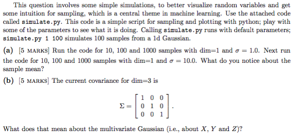
This question involves some simple simulations, to better visualize random variables and get some intuition for sampling, which is a central theme in machine learning. Use the attached code called \verb+simulate.py+. This code is a simple script for sampling and plotting with python; play with some of the parameters to see what it is doing. Calling \verb+simulate.py+ runs with default parameters; \verb+simulate.py 1 100+ simulates 100 samples from a 1d Gaussian.

\subquestion{5} Run the code for 10, 100 and 1000 samples with dim=1 and $\sigma = 1.0$. Next run the code for 10, 100 and 1000 samples with dim=1 and $\sigma = 10.0$. What do you notice about the sample mean?

\subquestion{5} The current covariance for dim=3 is % \begin{align*} \Sigma = \left[ \begin{array}{ccc} 1 & 0 & 0 \\ 0 & 1 & 0 \\ 0 & 0 & 1\end{array} ight] . \end{align*} % % What does that mean about the multivariate Gaussian (i.e., about $X$, $Y$ and $Z$)?

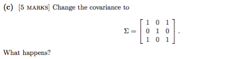
\subquestion{5} Change the covariance to % \begin{align*} \Sigma = \left[ \begin{array}{ccc} 1 & 0 & 1 \\ 0 & 1 & 0 \\ 1 & 0 & 1\end{array} ight] . \end{align*} % % What happens?

\question{30}

Suppose that the number of accidents occurring daily in a certain plant has a Poisson distribution with an unknown mean $\lambda$. Based on previous experience in similar industrial plants, suppose that our initial feelings about the possible value of $\lambda$ can be expressed by an exponential distribution with parameter $\theta=\tfrac{1}{2}$. That is, the prior density is % \begin{align*} f(\lambda)=\theta \textrm{e}^{-\theta\lambda} \end{align*} % % where $\lambda\in (0,\infty)$.

\subquestion{5} Before observing any data (any reported accidents), what is the most likely value for $\lambda$?

\subquestion{5} Now imagine there are 79 accidents over 9 days. Determine the maximum likelihood estimate of $\lambda$.

\subquestion{5} Again imagine there are 79 accidents over 9 days. Determine the maximum a posteriori (MAP) estimate of $\lambda$.

\subquestion{5} Imagine you now want to predict the number of accidents for tomorrow. How can you use the maximum likelihood estimate computed above? What about the MAP estimate? What would they predict?

\subquestion{5} For the MAP estimate, what is the purpose of the prior once we observe this data?

\subquestion{5} Look at the plots of some exponential distributions to better understand the prior chosen on $\lambda$. Imagine that now new safety measures have been put in place and you believe that the number of accidents per day should sharply decrease. How might you change $\theta$ to better reflect this new belief about the number of accidents?

\question{30}

Imagine that you would like to predict if your favorite table will be free at your favorite restaurant. The only additional piece of information you can collect, however, is if it is sunny or not sunny. % You collect paired samples from visit of the form (is sunny, is table free), where it is either sunny (1) or not sunny (0) and the table is either free (1) or not free(0).

\subquestion{10} How can this be formulated as a maximum likelihood problem?

\subquestion{10} Assume you have collected data for the last 10 days and computed the maximum likelihood solution to the problem formulated in (a). If it is sunny today, how would you predict if your table will be free?

\subquestion{10} Imagine now that you could further gather information about if it is morning, afternoon, or evening. How does this change the maximum likelihood problem?

\vspace{0.5cm} \begin{center} {\large \textbf{Homework policies:}} \end{center}

Your assignment will be submitted as a single pdf document and a zip file with code, on canvas. The questions must be typed; for example, in Latex, Microsoft Word, Lyx, etc. or must be written legibly and scanned. Images may be scanned and inserted into the document if it is too complicated to draw them properly. %Submit a single pdf document or, if you are attaching your code, %submit your code together with the typed (single) document as one .zip file. % All code (if applicable) should be turned in when you submit your assignment. Use Matlab, Python, R, Java or C.

Policy for late submission assignments: Unless there are legitimate circumstances, late assignments will be accepted up to 5 days after the due date and graded using the following rule:

\begin{enumerate} \itemsep0em \item[] on time: your score 1 \item[] 1 day late: your score 0.9 \item[] 2 days late: your score 0.7 \item[] 3 days late: your score 0.5 \item[] 4 days late: your score 0.3 \item[] 5 days late: your score 0.1 \end{enumerate}

For example, this means that if you submit 3 days late and get 80 points for your answers, your total number of points will be $80 \times 0.5 = 40$ points.

All assignments are individual, except when collaboration is explicitly allowed. All the sources used for problem solution must be acknowledged, e.g. web sites, books, research papers, personal communication with people, etc. Academic honesty is taken seriously; for detailed information see Indiana University Code of Student Rights, Responsibilities, and Conduct.

\begin{center} {\large \textbf{Good luck!}} \end{center}

\label{EndOfAssignment}%

\end{document}

This question involves some simple simulations, to better visualize random variables and get some intuition for sampling, which is a central theme in machine learning. Use the attached code called simulate.py. This code is a simple script for sampling and plotting with python; play with some of the parameters to see what it is doing. Calling simulate. py runs with default parameters; simulate .py 1 100 simulates 100 samples from a ld Gaussian. (a) 5 MARKs Run the code for 10, 100 and 1000 samples with dima 1 and a 1.0. Next run the code for 10, 100 and 1000 samples with dim i and or 10.0. What do you notice about the sample mean? (b) (5 MARKs] The current covariance for dima 3 is 1 0 0 s- o 1 0 0 0 1 What does that mean about the multivariate Gaussian (ie, about X, Y and Z)? This question involves some simple simulations, to better visualize random variables and get some intuition for sampling, which is a central theme in machine learning. Use the attached code called simulate.py. This code is a simple script for sampling and plotting with python; play with some of the parameters to see what it is doing. Calling simulate. py runs with default parameters; simulate .py 1 100 simulates 100 samples from a ld Gaussian. (a) 5 MARKs Run the code for 10, 100 and 1000 samples with dima 1 and a 1.0. Next run the code for 10, 100 and 1000 samples with dim i and or 10.0. What do you notice about the sample mean? (b) (5 MARKs] The current covariance for dima 3 is 1 0 0 s- o 1 0 0 0 1 What does that mean about the multivariate Gaussian (ie, about X, Y and Z)