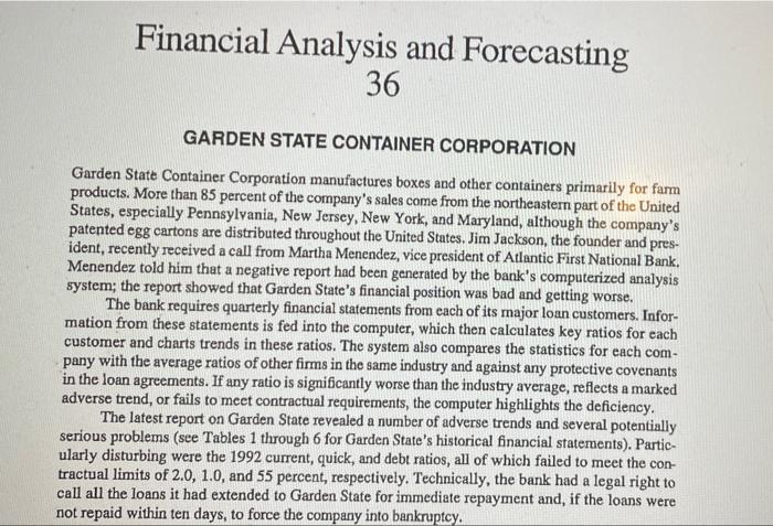
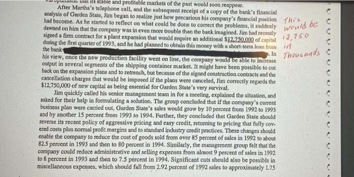
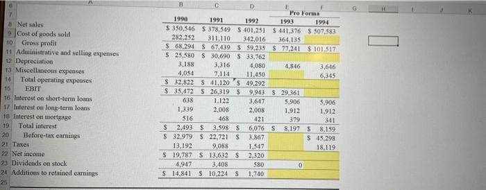
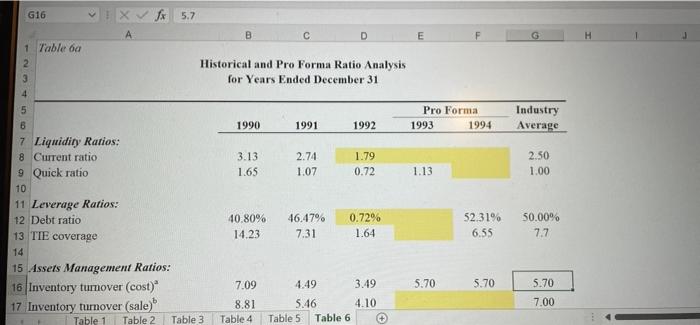
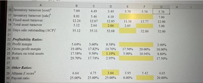
Financial Analysis and Forecasting 36 GARDEN STATE CONTAINER CORPORATION Garden State Container Corporation manufactures boxes and other containers primarily for farm products. More than 85 percent of the company's sales come from the northeastern part of the United States, especially Pennsylvania, New Jersey, New York, and Maryland, although the company's patented egg cartons are distributed throughout the United States. Jim Jackson, the founder and pres. ident, recently received a call from Martha Menendez, vice president of Atlantic First National Bank. Menendez told him that a negative report had been generated by the bank's computerized analysis system; the report showed that Garden State's financial position was bad and getting worse. The bank requires quarterly financial statements from each of its major loan customers. Infor- mation from these statements is fed into the computer, which then calculates key ratios for each customer and charts trends in these ratios. The system also compares the statistics for each com- pany with the average ratios of other firms in the same industry and against any protective covenants in the loan agreements. If any ratio is significantly worse than the industry average, reflects a marked adverse trend, or fails to meet contractual requirements, the computer highlights the deficiency. The latest report on Garden State revealed a number of adverse trends and several potentially serious problems (see Tables 1 through 6 for Garden State's historical financial statements). Partic- ularly disturbing were the 1992 current, quick, and debt ratios, all of which failed to meet the con- tractual limits of 2.0, 1.0, and 55 percent, respectively. Technically, the bank had a legal right to call all the loans it had extended to Garden State for immediate repayment and, if the loans were not repaid within ten days, to force the company into bankruptcy. canal de louns it had extended to Garden State for immediate repayment and, it the loans were not repaid within ten days, to force the company into bankruptcy. Martha hoped to avoid calling the loans if at all possible, as she knew this would back Gar- den State into a comer from which it might not be able to emerge. Still, her own bank's examiners had recently become highly sensitive to the issue of problem loans, because the recent spate of bank failures had forced regulators to become more strict in their examination of bank loan portfo- lios and to demand earlier identification of potential repayment problems. One measure of the quality of a loan is the Altman 2 score, which for Garden State was 3.04 for 1992, slightly below the 3.20 minimum that Martha's bank uses to differentiate strong firms with little likelihood of bankruptcy in the next two years from those deemed likely to go into default. This will put the bank under increased pressure to reclassify Garden State's loans as "problem loans," to set up a reserve to cover potential losses, and to take whatever steps are necessary to reduce the bank's exposure. Setting up the loss reserve would have a negative effect on the bank's profits and reflect badly on Martha's performance. To keep Garden State's loan from being reclassified as a "problem loan," the Senior Loan Committee will require strong and convincing evidence that the company's present difficulties are a only temporary. Therefore, it must be shown that appropriate actions to overcome the problems have been taken and that the chances of reversing the adverse trends are realistically good. Martha now has the task of collecting the necessary information, evaluating its implications, and preparing a recommendation for action. The recession that plagued the U.S. economy in the early 1990s caused severe, though hope- fully temporary, problems for companies like Garden State. On top of this, disastrous droughts for two straight summers had devastated vegetable crops in the area, leading to a drastic curtailment of demand for produce shipping containers. In light of the softening demand, Garden State had aggres- sively reduced prices in 1991 and 1992 to stimulate sales. Higher sales, the company believed, would allow it to realize greater economies of scale in production and to ride the learning, or experience, curve down to a lower cost position. Garden State's management had full confidence that normal weather and national economic policies would revive the ailing economy and that the downturn in demand would be only a short-term problem. Consequently, production continued unabated, and inventories increased sharply. In a further effort to reduce inventory, Garden State relaxed its credit standards in early 1992 and improved its already favorable credit terms. As a result, sales growth did remain high by indus- try standards through the third quarter of 1992, but not high enough to keep inventories from con tinuing to rise. Further, the credit policy changes had caused accounts receivable to increase dramatically by late 1992. To finance its rising inventories and receivables, Garden State turned to the bank for a long- term loan in 1991 and also increased its short-term credit lines in both 1991 and 1992. However, this expanded credit was insufficient to cover the asset expansion, so the company began to delay pay- ments of its accounts payable until the second late notice had been received. Management realized that this was not a particularly wise decision for the long run, but they did not think it would be necessary to follow the policy for very long-the 1992 summer vegetable crop looked like a record breaker, and it was unlikely that a severe drought would again hurt the crop. They also predicted that the national economy would pull out of the weak growth scenario in late 1992. Thus, the company was optimistic that its stable and profitable markets of the past would soon reappear. C C In Thousands o URL is stable and profitable markets of the past would soon reappear. After Martha's telephone call, and the subsequent receipt of a copy of the bank's financial analysis of Garden State, Jim began to realize just how precarious his company's financial position thi's to be dawned on him that the company was in even more trouble than the bank imagined. Jim had recently signed a 12,750 during the first quarter of 1993, and he had planned to obtain this money with a short-term loan from in the bank his view, once the new production facility went on line, the company would be able to increase output in several segments of the shipping container market. It might have been possible to cut back on the expansion plans and to retrench, but because of the signed construction contracts and the cancellation charges that would be imposed if the plans were canceled, Jim correctly regards the $12,750,000 of new capital as being essential for Garden State's very survival. Jim quickly called his senior management team in for a meeting, explained the situation, and asked for their help in formulating a solution. The group concluded that if the company's current business plan were carried out, Garden State's sales would grow by 10 percent from 1992 to 1993 and by another 15 percent from 1993 to 1994. Further, they concluded that Garden State should reverse its recent policy of aggressive pricing and easy credit, returning to pricing that fully cov- ered costs plus normal profit margins and to standard industry credit practices. These changes should enable the company to reduce the cost of goods sold from over 85 percent of sales in 1992 to about 82.5 percent in 1993 and then to 80 percent in 1994. Similarly, the management group felt that the company could reduce administrative and selling expenses from almost 9 percent of sales in 1992 to 8 percent in 1993 and then to 7.5 percent in 1994. Significant cuts should also be possible in miscellaneous expenses, which should fall from 2.92 percent of 1992 sales to approximately 1.75 percent of sales in 1993 and to 1.25 percent in 1994. These cost reductions represented "trimming the fat," so they were not expected to degrade the quality of the firm's products or the effectiveness of its sales efforts. Further, to appease suppliers, future bills would be paid more promptly, and to convince the bank how serious management is about correcting the company's problems, cash div. idends would be eliminated until the firm regains its financial health. Assume that Jim has hired you as a consultant to first verify the bank's evaluation of the company's current financial situation and then to put together a forecast of Garden State's expected performance for 1993 and 1994. Jim asks you to develop some figures that ignore the possibility of a reduction in the credit lines and that assume the bank will increase the line of credit by the $12,750,000 needed for the expansion and supporting working capital. Also, you and Jim do not expect the level of interest rates to change substantially over the two-year forecast period; how- ever, you both think that the bank will charge 12 percent on both the additional short-term loan, if it is granted, and on the existing short-term loans, if they are extended. The assumed 40 percent com bined federal and state tax rate should also hold for two years. Finally, if the bank cooperates, and if Jim is able to turn the company around, the P/E ratio should be 12 in 1993 and should rise to 14 in 1994. Your first task is to construct a set of pro forma financial statements that Jim and the rest of the Garden State management team can use to assess the company's position and also to convince Martha that her bank's loan is safe, provided the bank will extend the firm's line of credit. Then, you must present your projections, with recommendations for future action to Garden State's manage- ment and to Martha. To prepare for your presentations, answer the following questions, keeping in mind that the Garden State managers and particularly, Martha and her bosses, could ask you some tough questions about your analysis and recommendations. Put another way, the following questions are designed to help you focus on the issues, but they are not meant to be a complete and exhaus- tive list of all the relevant points. 4. Now complete the tables to develop pro forma financial statements for 1993 and 1994. For these calculations, assume that the bank is willing to maintain the present credit lines and to grant an additional $12,750,000 of short-term credit on January 1, 1993. In the analysis, take account of the amounts of inventory and accounts receivable that would be carried if inventory utilization (based on the cost of goods sold) and days sales outstanding were set at industry-average levels. Also, assume in your forecast that all of Garden State's plans and predictions concerning sales and expenses materialize and that the firm pays no cash dividends during the forecast 3 4 5 for Years Ended December 31 (in Thousands of Dollars) Pro Forma 1993 1994 1990 1991 1992 6 7 8 Assets: 9 Cash and marketable securities 0 Accounts receivable 1 Inventory 2 Current assets 3 Land, buildings, plant, and equipment Accumulated depreciation 5 Net fixed assets = Total assets $ 9.901 $ 7,363 $ 6,550 34,196 36,924 58,714 39.791 69,361 97,984 $ 83,888 $ 113,647 S 163,249 $ 34,634 $ 39,195 $ 44,604 $ 57,036 S 58,746 (5,992) (9,308) (13,388) (18,234) (21.880) $ 28,642 $ 29,887 $ 31,216 $ 38,802 $ 36,866 $ 112,530 $ 143,534 $ 194,465 $ 215,375 Liabilities and Equities: Short-term bank loans $ 6,376 $ 10,200 $ 36.466 Table 1 Table 2 Table 3 Table 4 Table 5 Table 6 F G G H B D E $112,530 $ 143,534 $ 194,465 S 215,375 A 16 Total assets 17 18 Liabilities and Equities: 19 Short-term bank loans 20 Accounts payable 21 Accruals 22 Current liabilities 23 Long-term bank loans 24 Mortgage 25 Long-term debt 26 Total liabilities 27 Common stock 28 Retained earnings 29 Total equity 30 Total liabilities and equity 31 32 S 6,376 $ 10,200 $ 36,466 13,528 21,012 39,996 31,990 33,590 6,886 10,200 14.662 18,602 23,252 $ 26,790 $ 41.412 S 91.124 $ 13,388 $ 20,082 $ 20,082 $ 20,082 $ 20,082 5,738 5,202 4,680 4,208 3,788 $ 19.126 S 25.284 $ 24.762 $ 24.290 $23.870 $ 45,916 S 66.696 $ 115,886 $ 46,538 $ 46,538 $ 46,538 $ 46,538 $ 46,538 20,076 30,300 32,041 66,614 $ 76,838 $ 78.579 $ 112,530 $ 143,534 $ 194,465 1 # Net sales 9 Cost of goods sold 10 Gross profit 11 Administrative and selling expenses 12 Depreciation 13 Miscellaneous expenses 14 Total operating expenses 15 EBIT 16 Interest on short-term loans 17 Interest on long-term loans 18 Interest on mortgage 19 Total interest 20 Before-tax earnings 21 Taxes 22 Net income 23 Dividends on stock 24 Additions to retained eamings 25 B D E Pro Forma 1990 1991 1992 1993 1994 $ 350,546 $ 378,549 $ 401,251 $ 411.376 S 507,583 282,252 311,110 342,016 364.135 $ 68,294 S 67.439 3 59.235 S 77.241 $ 101.517 $ 25,580 $30,690 533,762 3.188 3.316 4,080 4,846 3,646 4,054 7,114 11.450 6,345 $ 32,822 S 41,120 S 49,292 $ 35.472 S 26,319S 9,943 $ 29,361 638 1.122 3,647 5,906 5,906 1,339 2.008 2,008 1.912 1,912 516 468 421 379 341 $ 2.493 $ 3.5985 6,076 S 8,197 5 8,159 $32.979 $ 22,721 S 3.867 $ 45,298 13,192 9.088 1.547 18.119 $ 19,787 S. 13,632 $ 2.320 4.947 3,408 580 0 S 14,841 $ 10,224 S 1,740 G16 fx 5.7 B D E H 1 Table 60 2 Historical and Pro Forma Ratio Analysis for Years Ended December 31 Pro Forma 1993 1994 Industry Average 1990 1991 1992 3.13 1.65 2.74 1.07 1.79 0.72 2.50 1.00 1.13 5 6 7 Liquidity Ratios: 8 Current ratio 9 Quick ratio 10 11 Leverage Ratios: 12 Debt ratio 13 TIE coverage 14 15 Assets Management Ratios: 16 Inventory turnover (cost) 17 Inventory turnover (sale) Table 1 Table 2 Table 3 40.80% 14.23 46.47% 7.31 0.72% 1.64 52.31% 6.55 50.00% 7.7 7.09 4.49 3.49 5.70 5.70 5.70 7.00 8.81 Table 4 5.46 4.10 Table 5 Table 6 B F G D 3.49 E 5.70 5.70 5.70 7.09 8.81 12.24 3.12 35.12 4.49 5.46 12.67 2.64 13.77 4.10 12.85 2.06 52.68 11.38 2.05 7.00 12.00 3.00 32.00 35.11 32.00 16 Inventory turnover (cost) 17 Inventory turnover (sale) 18 Fixed asset tumover 19 Total asset turnover 20 Days sale outstanding (ACP) 21 22 Profitability Ratios: 23 Profit margin 24 Gross profit margin 25 Return on total assets 26 ROE 27 28 Other Ratios: 29 Altman Z score 30 Payout ratio 5.64% 19.48% 17.58% 29.70% 3.60% 17.82% 9.50% 17.74% 0.58% 14.76% 1.19% 2.95% 17.50% 5.90% 20.00% 10.94% 2.90% 18.00% 8.80% 17.50% 5.42 6.64 25.00% 4.75 25.00 3.04 25.00% 3.95 0.00% 4.65 20.00% Financial Analysis and Forecasting 36 GARDEN STATE CONTAINER CORPORATION Garden State Container Corporation manufactures boxes and other containers primarily for farm products. More than 85 percent of the company's sales come from the northeastern part of the United States, especially Pennsylvania, New Jersey, New York, and Maryland, although the company's patented egg cartons are distributed throughout the United States. Jim Jackson, the founder and pres. ident, recently received a call from Martha Menendez, vice president of Atlantic First National Bank. Menendez told him that a negative report had been generated by the bank's computerized analysis system; the report showed that Garden State's financial position was bad and getting worse. The bank requires quarterly financial statements from each of its major loan customers. Infor- mation from these statements is fed into the computer, which then calculates key ratios for each customer and charts trends in these ratios. The system also compares the statistics for each com- pany with the average ratios of other firms in the same industry and against any protective covenants in the loan agreements. If any ratio is significantly worse than the industry average, reflects a marked adverse trend, or fails to meet contractual requirements, the computer highlights the deficiency. The latest report on Garden State revealed a number of adverse trends and several potentially serious problems (see Tables 1 through 6 for Garden State's historical financial statements). Partic- ularly disturbing were the 1992 current, quick, and debt ratios, all of which failed to meet the con- tractual limits of 2.0, 1.0, and 55 percent, respectively. Technically, the bank had a legal right to call all the loans it had extended to Garden State for immediate repayment and, if the loans were not repaid within ten days, to force the company into bankruptcy. canal de louns it had extended to Garden State for immediate repayment and, it the loans were not repaid within ten days, to force the company into bankruptcy. Martha hoped to avoid calling the loans if at all possible, as she knew this would back Gar- den State into a comer from which it might not be able to emerge. Still, her own bank's examiners had recently become highly sensitive to the issue of problem loans, because the recent spate of bank failures had forced regulators to become more strict in their examination of bank loan portfo- lios and to demand earlier identification of potential repayment problems. One measure of the quality of a loan is the Altman 2 score, which for Garden State was 3.04 for 1992, slightly below the 3.20 minimum that Martha's bank uses to differentiate strong firms with little likelihood of bankruptcy in the next two years from those deemed likely to go into default. This will put the bank under increased pressure to reclassify Garden State's loans as "problem loans," to set up a reserve to cover potential losses, and to take whatever steps are necessary to reduce the bank's exposure. Setting up the loss reserve would have a negative effect on the bank's profits and reflect badly on Martha's performance. To keep Garden State's loan from being reclassified as a "problem loan," the Senior Loan Committee will require strong and convincing evidence that the company's present difficulties are a only temporary. Therefore, it must be shown that appropriate actions to overcome the problems have been taken and that the chances of reversing the adverse trends are realistically good. Martha now has the task of collecting the necessary information, evaluating its implications, and preparing a recommendation for action. The recession that plagued the U.S. economy in the early 1990s caused severe, though hope- fully temporary, problems for companies like Garden State. On top of this, disastrous droughts for two straight summers had devastated vegetable crops in the area, leading to a drastic curtailment of demand for produce shipping containers. In light of the softening demand, Garden State had aggres- sively reduced prices in 1991 and 1992 to stimulate sales. Higher sales, the company believed, would allow it to realize greater economies of scale in production and to ride the learning, or experience, curve down to a lower cost position. Garden State's management had full confidence that normal weather and national economic policies would revive the ailing economy and that the downturn in demand would be only a short-term problem. Consequently, production continued unabated, and inventories increased sharply. In a further effort to reduce inventory, Garden State relaxed its credit standards in early 1992 and improved its already favorable credit terms. As a result, sales growth did remain high by indus- try standards through the third quarter of 1992, but not high enough to keep inventories from con tinuing to rise. Further, the credit policy changes had caused accounts receivable to increase dramatically by late 1992. To finance its rising inventories and receivables, Garden State turned to the bank for a long- term loan in 1991 and also increased its short-term credit lines in both 1991 and 1992. However, this expanded credit was insufficient to cover the asset expansion, so the company began to delay pay- ments of its accounts payable until the second late notice had been received. Management realized that this was not a particularly wise decision for the long run, but they did not think it would be necessary to follow the policy for very long-the 1992 summer vegetable crop looked like a record breaker, and it was unlikely that a severe drought would again hurt the crop. They also predicted that the national economy would pull out of the weak growth scenario in late 1992. Thus, the company was optimistic that its stable and profitable markets of the past would soon reappear. C C In Thousands o URL is stable and profitable markets of the past would soon reappear. After Martha's telephone call, and the subsequent receipt of a copy of the bank's financial analysis of Garden State, Jim began to realize just how precarious his company's financial position thi's to be dawned on him that the company was in even more trouble than the bank imagined. Jim had recently signed a 12,750 during the first quarter of 1993, and he had planned to obtain this money with a short-term loan from in the bank his view, once the new production facility went on line, the company would be able to increase output in several segments of the shipping container market. It might have been possible to cut back on the expansion plans and to retrench, but because of the signed construction contracts and the cancellation charges that would be imposed if the plans were canceled, Jim correctly regards the $12,750,000 of new capital as being essential for Garden State's very survival. Jim quickly called his senior management team in for a meeting, explained the situation, and asked for their help in formulating a solution. The group concluded that if the company's current business plan were carried out, Garden State's sales would grow by 10 percent from 1992 to 1993 and by another 15 percent from 1993 to 1994. Further, they concluded that Garden State should reverse its recent policy of aggressive pricing and easy credit, returning to pricing that fully cov- ered costs plus normal profit margins and to standard industry credit practices. These changes should enable the company to reduce the cost of goods sold from over 85 percent of sales in 1992 to about 82.5 percent in 1993 and then to 80 percent in 1994. Similarly, the management group felt that the company could reduce administrative and selling expenses from almost 9 percent of sales in 1992 to 8 percent in 1993 and then to 7.5 percent in 1994. Significant cuts should also be possible in miscellaneous expenses, which should fall from 2.92 percent of 1992 sales to approximately 1.75 percent of sales in 1993 and to 1.25 percent in 1994. These cost reductions represented "trimming the fat," so they were not expected to degrade the quality of the firm's products or the effectiveness of its sales efforts. Further, to appease suppliers, future bills would be paid more promptly, and to convince the bank how serious management is about correcting the company's problems, cash div. idends would be eliminated until the firm regains its financial health. Assume that Jim has hired you as a consultant to first verify the bank's evaluation of the company's current financial situation and then to put together a forecast of Garden State's expected performance for 1993 and 1994. Jim asks you to develop some figures that ignore the possibility of a reduction in the credit lines and that assume the bank will increase the line of credit by the $12,750,000 needed for the expansion and supporting working capital. Also, you and Jim do not expect the level of interest rates to change substantially over the two-year forecast period; how- ever, you both think that the bank will charge 12 percent on both the additional short-term loan, if it is granted, and on the existing short-term loans, if they are extended. The assumed 40 percent com bined federal and state tax rate should also hold for two years. Finally, if the bank cooperates, and if Jim is able to turn the company around, the P/E ratio should be 12 in 1993 and should rise to 14 in 1994. Your first task is to construct a set of pro forma financial statements that Jim and the rest of the Garden State management team can use to assess the company's position and also to convince Martha that her bank's loan is safe, provided the bank will extend the firm's line of credit. Then, you must present your projections, with recommendations for future action to Garden State's manage- ment and to Martha. To prepare for your presentations, answer the following questions, keeping in mind that the Garden State managers and particularly, Martha and her bosses, could ask you some tough questions about your analysis and recommendations. Put another way, the following questions are designed to help you focus on the issues, but they are not meant to be a complete and exhaus- tive list of all the relevant points. 4. Now complete the tables to develop pro forma financial statements for 1993 and 1994. For these calculations, assume that the bank is willing to maintain the present credit lines and to grant an additional $12,750,000 of short-term credit on January 1, 1993. In the analysis, take account of the amounts of inventory and accounts receivable that would be carried if inventory utilization (based on the cost of goods sold) and days sales outstanding were set at industry-average levels. Also, assume in your forecast that all of Garden State's plans and predictions concerning sales and expenses materialize and that the firm pays no cash dividends during the forecast 3 4 5 for Years Ended December 31 (in Thousands of Dollars) Pro Forma 1993 1994 1990 1991 1992 6 7 8 Assets: 9 Cash and marketable securities 0 Accounts receivable 1 Inventory 2 Current assets 3 Land, buildings, plant, and equipment Accumulated depreciation 5 Net fixed assets = Total assets $ 9.901 $ 7,363 $ 6,550 34,196 36,924 58,714 39.791 69,361 97,984 $ 83,888 $ 113,647 S 163,249 $ 34,634 $ 39,195 $ 44,604 $ 57,036 S 58,746 (5,992) (9,308) (13,388) (18,234) (21.880) $ 28,642 $ 29,887 $ 31,216 $ 38,802 $ 36,866 $ 112,530 $ 143,534 $ 194,465 $ 215,375 Liabilities and Equities: Short-term bank loans $ 6,376 $ 10,200 $ 36.466 Table 1 Table 2 Table 3 Table 4 Table 5 Table 6 F G G H B D E $112,530 $ 143,534 $ 194,465 S 215,375 A 16 Total assets 17 18 Liabilities and Equities: 19 Short-term bank loans 20 Accounts payable 21 Accruals 22 Current liabilities 23 Long-term bank loans 24 Mortgage 25 Long-term debt 26 Total liabilities 27 Common stock 28 Retained earnings 29 Total equity 30 Total liabilities and equity 31 32 S 6,376 $ 10,200 $ 36,466 13,528 21,012 39,996 31,990 33,590 6,886 10,200 14.662 18,602 23,252 $ 26,790 $ 41.412 S 91.124 $ 13,388 $ 20,082 $ 20,082 $ 20,082 $ 20,082 5,738 5,202 4,680 4,208 3,788 $ 19.126 S 25.284 $ 24.762 $ 24.290 $23.870 $ 45,916 S 66.696 $ 115,886 $ 46,538 $ 46,538 $ 46,538 $ 46,538 $ 46,538 20,076 30,300 32,041 66,614 $ 76,838 $ 78.579 $ 112,530 $ 143,534 $ 194,465 1 # Net sales 9 Cost of goods sold 10 Gross profit 11 Administrative and selling expenses 12 Depreciation 13 Miscellaneous expenses 14 Total operating expenses 15 EBIT 16 Interest on short-term loans 17 Interest on long-term loans 18 Interest on mortgage 19 Total interest 20 Before-tax earnings 21 Taxes 22 Net income 23 Dividends on stock 24 Additions to retained eamings 25 B D E Pro Forma 1990 1991 1992 1993 1994 $ 350,546 $ 378,549 $ 401,251 $ 411.376 S 507,583 282,252 311,110 342,016 364.135 $ 68,294 S 67.439 3 59.235 S 77.241 $ 101.517 $ 25,580 $30,690 533,762 3.188 3.316 4,080 4,846 3,646 4,054 7,114 11.450 6,345 $ 32,822 S 41,120 S 49,292 $ 35.472 S 26,319S 9,943 $ 29,361 638 1.122 3,647 5,906 5,906 1,339 2.008 2,008 1.912 1,912 516 468 421 379 341 $ 2.493 $ 3.5985 6,076 S 8,197 5 8,159 $32.979 $ 22,721 S 3.867 $ 45,298 13,192 9.088 1.547 18.119 $ 19,787 S. 13,632 $ 2.320 4.947 3,408 580 0 S 14,841 $ 10,224 S 1,740 G16 fx 5.7 B D E H 1 Table 60 2 Historical and Pro Forma Ratio Analysis for Years Ended December 31 Pro Forma 1993 1994 Industry Average 1990 1991 1992 3.13 1.65 2.74 1.07 1.79 0.72 2.50 1.00 1.13 5 6 7 Liquidity Ratios: 8 Current ratio 9 Quick ratio 10 11 Leverage Ratios: 12 Debt ratio 13 TIE coverage 14 15 Assets Management Ratios: 16 Inventory turnover (cost) 17 Inventory turnover (sale) Table 1 Table 2 Table 3 40.80% 14.23 46.47% 7.31 0.72% 1.64 52.31% 6.55 50.00% 7.7 7.09 4.49 3.49 5.70 5.70 5.70 7.00 8.81 Table 4 5.46 4.10 Table 5 Table 6 B F G D 3.49 E 5.70 5.70 5.70 7.09 8.81 12.24 3.12 35.12 4.49 5.46 12.67 2.64 13.77 4.10 12.85 2.06 52.68 11.38 2.05 7.00 12.00 3.00 32.00 35.11 32.00 16 Inventory turnover (cost) 17 Inventory turnover (sale) 18 Fixed asset tumover 19 Total asset turnover 20 Days sale outstanding (ACP) 21 22 Profitability Ratios: 23 Profit margin 24 Gross profit margin 25 Return on total assets 26 ROE 27 28 Other Ratios: 29 Altman Z score 30 Payout ratio 5.64% 19.48% 17.58% 29.70% 3.60% 17.82% 9.50% 17.74% 0.58% 14.76% 1.19% 2.95% 17.50% 5.90% 20.00% 10.94% 2.90% 18.00% 8.80% 17.50% 5.42 6.64 25.00% 4.75 25.00 3.04 25.00% 3.95 0.00% 4.65 20.00%