For a homework question, we have to plot the solution to a diffusion problem at multiple time points. Here is the question: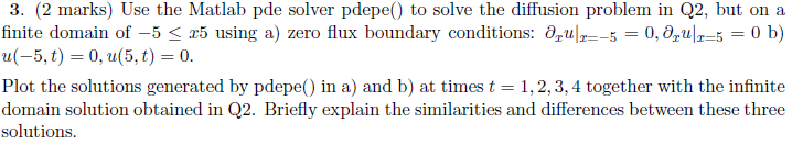

Here is my answer to the Q2 mentioned:

x = -5:0.05:5;

t1 = 0.01; t2 = 0.1; t3 = 1;

y1 = 0.5*(erf((x+1)/sqrt(4*t1))-erf((x-1)/sqrt(4*t1))); y2 = 0.5*(erf((x+1)/sqrt(4*t2))-erf((x-1)/sqrt(4*t2))); y3 = 0.5*(erf((x+1)/sqrt(4*t3))-erf((x-1)/sqrt(4*t3)));

plot(x, y1, x, y2, x, y3) xlabel('x') ylabel('u(x,t)') title('Plotting for three time points') legend('t=0.01','t=0.1','t=1')

And I am wondering how to do question 3. Here are the barebones of the code, slightly adjusted from a previous question:

function ass3q3 close all m = 0; x = linspace(0,1,20); t = linspace(0,0.3,4);

sol = pdepe(m,@pdex1pde,@pdex1ic,@pdex1bc,x,t); u = sol(:,:,1);

% Calculating the theoretical solution: t1 = 0.01; t2 = 0.1; t3 = 1;

y = 0.5*(erf((x+1)/sqrt(4*t1))-erf((x-1)/sqrt(4*t1))); z = 0.5*(erf((x+1)/sqrt(4*t2))-erf((x-1)/sqrt(4*t2))); w = 0.5*(erf((x+1)/sqrt(4*t3))-erf((x-1)/sqrt(4*t3)));

figure subplot(2,2,1); hold on plot(x,u(1,:),'*') plot(x,y+z+w,'-')

% A solution profile can also be illuminating end % -------------------------------------------------------------- %this subfunction defines the pde, for the diffusion equation see the pdepe %help [age for the matlab definition of these terms. function [c,f,s] = pdex1pde(x,t,u,DuDx) c = 1; f = DuDx; s = 0; end % -------------------------------------------------------------- %this subfunction defines initial condition u(x,0) function u0 = pdex1ic(x)

if abs(x)

end % -------------------------------------------------------------- %this function defines the boundary condition, see the pdepe help page %for the matlab definition of these terms function [pl,ql,pr,qr] = pdex1bc(xl,ul,xr,ur,t) %zero fluxing boundary pl = ul; ql = 0; pr = ur; qr = 0; end

3. (2 marks) Use the Matlab pde solver pdepe) to solve the diffusion problem in Q2, but on a finite domain of -5 S r5 using a) zero flx boundary conditions: Oru--5-0,u b) u(-5, t) 0, u(5,t)0 Plot the solutions generated by pdepe() in a) and b) at times t 1, 2, 3, 4 together with the infinite domain solution obtained in Q2. Briefly explain the similarities and differences between these three solutions 3. (2 marks) Use the Matlab pde solver pdepe) to solve the diffusion problem in Q2, but on a finite domain of -5 S r5 using a) zero flx boundary conditions: Oru--5-0,u b) u(-5, t) 0, u(5,t)0 Plot the solutions generated by pdepe() in a) and b) at times t 1, 2, 3, 4 together with the infinite domain solution obtained in Q2. Briefly explain the similarities and differences between these three solutions