For reference from P1:

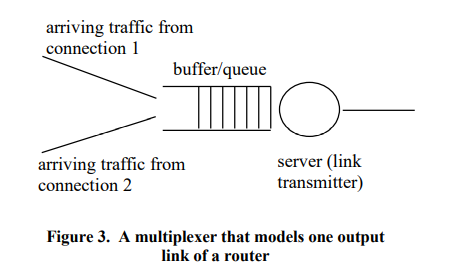
Problem 2 (20 points). Instead of specifying the starting and ending times of packet transmission (e.g., Problem 1 (e)), an alternative way of describing the traffic generating process is to think the traffic as a bit stream. This continuous approximation of the packet generating process is called the fluid model or the fluid approximation. One can also make a simple model to understand each output link of a router. This is illustrated in Figure 3. The buffer in the figure accepts and queues data (either packets or bit stream) from a number of connections (i.e., sender-receiver pairs). The queue is serviced when the output link transmits the data. This abstract model is called a multiplexer.

Question Itself:

Suppose one bit stream arrives at a buffer. The rate of the bit stream is a periodic function of time with period T = 1 second. During [0, T/4], the rate is equal to 10 Mbps and during (T/4, T), it is equal to zero. A transmitter with rate R bps serves the buffer by sending the bits whenever available.

(a) Draw a diagram that shows the occupancy of the buffer as a function of time, for different ranges of values for R.

(b) What is the minimum value R0 of R so that this occupancy does not keep growing?

(c) For 10 R R0, express the average delay D(R) per bit as a function of R.

(d) For 10 R R0, express the average buffer occupancy (over time) L(R) as a function of R.

(e) Show that L(R) = l D(R), where l = 2.5 Mbps is the average arrival rate of the bits. This is an example of the Littles Formula.

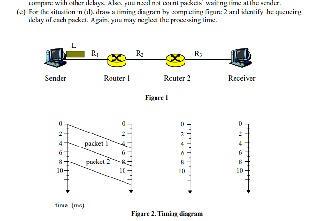
compare with other delays. Also, you need not count packets' waiting time at the sender. (e) For the situation in (d), draw a timing diagram by completing figure 2 and identify the queueing delay of each packet. Again, you may neglect the processing time. L RI R2 R3 Sender Router 1 Router 2 Receiver Figure 1 0 0 2 2 2 packet 1 4 0 2+ 4 6+ 8 10 4 6 6 6 packet 2 & 8 8 10 10 10 time (ms) Figure 2. Timing diagram arriving traffic from connection 1 buffer/queue IO arriving traffic from connection 2 server (link transmitter) Figure 3. A multiplexer that models one output link of a router compare with other delays. Also, you need not count packets' waiting time at the sender. (e) For the situation in (d), draw a timing diagram by completing figure 2 and identify the queueing delay of each packet. Again, you may neglect the processing time. L RI R2 R3 Sender Router 1 Router 2 Receiver Figure 1 0 0 2 2 2 packet 1 4 0 2+ 4 6+ 8 10 4 6 6 6 packet 2 & 8 8 10 10 10 time (ms) Figure 2. Timing diagram arriving traffic from connection 1 buffer/queue IO arriving traffic from connection 2 server (link transmitter) Figure 3. A multiplexer that models one output link of a router