Question
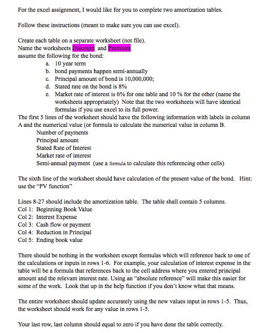
For the excel assignment, I would like for you to complete two amortization tables. Follow these instructions (meant to make sure you can use excel).
For the excel assignment, I would like for you to complete two amortization tables.
Follow these instructions (meant to make sure you can use excel).
Create each table on a separate worksheet (not file).
Name the worksheets Discount and Premium
assume the following for the bond:
(a) 10 year term
(b) bond payments happen semi-annually
(c) Principal amount of bond is 10,000,000;
(d) Stated rate on the bond is 8%
(e) Market rate of interest is 6% for one table and 10 % for the other (name the worksheets appropriately) Note that the two worksheets will have identical formulas if you use excel to its full power.
The first 5 lines of the worksheet should have the following information with labels in column A and the numerical value (or formula to calculate the numerical value in column B.
(a) Number of payments
(b) Principal amount
(c) Stated Rate of Interest
(d) Market rate of interest
(e) Semi-annual payment (use a formula to calculate this referencing other cells)
The sixth line of the worksheet should have calculation of the present value of the bond. Hint: use the PV function
Lines 8-27 should include the amortization table. The table shall contain 5 columns.
Col 1: Beginning Book Value
Col 2: Interest Expense
Col 3: Cash flow or payment
Col 4: Reduction in Principal
Col 5: Ending book value
There should be nothing in the worksheet except formulas which will reference back to one of the calculations or inputs in rows 1-6. For example, your calculation of interest expense in the table will be a formula that references back to the cell address where you entered principal amount and the relevant interest rate. Using an absolute reference will make this easier for some of the work. Look that up in the help function if you dont know what that means.
The entire worksheet should update accurately using the new values input in rows 1-5. Thus, the worksheet should work for any value in rows 1-5.
Your last row, last column should equal to zero if you have done the table correctly.
Step by Step Solution
There are 3 Steps involved in it
Step: 1

Get Instant Access to Expert-Tailored Solutions
See step-by-step solutions with expert insights and AI powered tools for academic success
Step: 2

Step: 3

Ace Your Homework with AI
Get the answers you need in no time with our AI-driven, step-by-step assistance
Get Started


