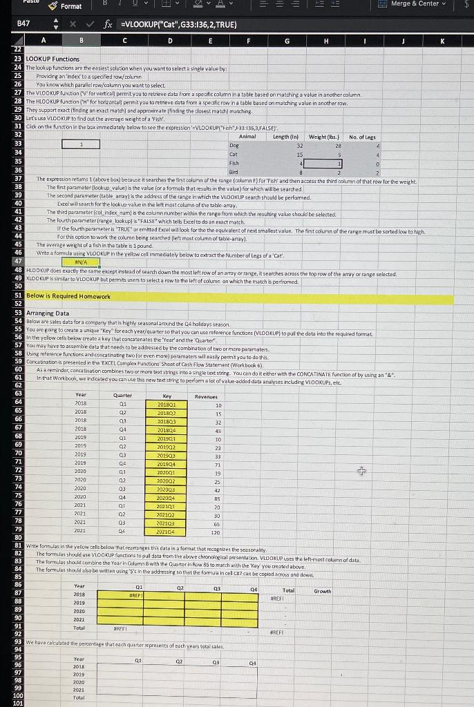
& Format == Merge & Center B47 X fx =VLOOKUP("Cat",G33:136,2, TRUE) K S A B C D E F G . J 22 23 LOOKUP Functions 24 The lookup functions are the easiest solution when you want to select a single value by: 25 Providing an 'index to a specified row/column 26 You know which parallel raw/column you want to select 27 The VLOOKUP Iunction('V'far vert call pemit you to retrieve data from a specific calumn in a table based on matching a value in another column. 28 The HLOOKUP function ('H' for horizontal perint you to retrieve data from a specific row na table based ori matching value in another row. 29 They support exact finding an exact match) and approximate finding the closest match matching 30 Let's & VLOOKUP to find out the average weight of a 'Fish 31 Click on the function in the bux immediately below to see the expression VLOOKUP("Fish',33:135,3,FALSEY 32 Animal Length (in) Weight (lbs.) No. of Legs 33 1 Doe 32 28 4 34 Cat 15 4 4 35 Fkh 1 0 36 Bird 8 2 37 The expression retums 1 (above box) because it searches the first column of the range (column F) for Fishy and then access the third column of that row for the weight 38 The first parameter lookup value) is the value (ar a formula that results in the value) for which will be searcted. 39 The second parameter (table array) is the address of the range in which the VLOOKUP search should be performed 40 Excel wil search for the lockup-value in the left most column of the table array 41 The third parameter icoLindex num) is the column number within the range from which the resulting value should be selected 42 The fourth parameter lange lookup) "FALSE" which tells Excel to do an act match. 43 If the fourth parameter is 'TRUE' or emitted Excel wil look for the the equivalent of next smallest value. The first column of the range must be sorted low to high 44 For this option to work the column being searched left most column of table array). 45 The average weight of a fish in the tables 1 pound 46 Write a fomula using VLOOKUP in the yellow cell immediatey below to extract the Number of Legs of a Cat 47 AN/A 48 HLOOKUP does exactly the same except instead of search down the most left row of an array or range, it searches across the top row of the array or range selected. 49 XLOOKUP is similar to VLOOKUP but permits users to select a row to the left of column on which the match is perfomed. 50 51 Below is Required Homework 52 53 Arranging Data 54 Below are sales data for a company that is highly seasonal around the 04 holdays season. 55 You are going to create a unique "Key" for each year/quarter so that you can use rotererce functions (VLOOKUP) to pull the data into the required formal 56 in the yelow cells below create a key that concatenates the 'Year' and the Quarter 57 You may beve to assemble data that needs to be addressed by the combination of two or more parameters 58 Using reference functions and conca tinating two for even more) paramaters wil easily permit you to do this 59 Conca tination is presented in the 'EXCEL Complex Functions'Sheat of Cash Flow Statement (Workbook 6). 60 As a reminder, conca tination combines two or more text strings into a single text string. You can do it either with the CONCATINATE function of by using an "& 61 In that Workbook, we indicated you can use this new text string to perform a lot of value-added data analyses including VLOOKUP, etc. 62 63 Year Quarter Key Revenues 64 2008 01 201801 10 65 2018 02 201802 15 66 2018 023 201803 32 67 2018 04 201804 45 68 2015 01 201901 10 69 2019 Q2 201902 23 70 2019 03 201993 33 71 2019 C4 201904 71 72 2020 01 202001 19 73 7020 92 202002 25 74 2020 99 202008 42 75 2020 04 202004 85 76 2021 01 200101 20 77 2001 Q2 202102 30 78 2021 Q3 202103 65 79 2021 04 202104 120 80 81 Write formulas in the yelow cels below that rearrange this data in a format that recognizes the seasonality 82 The formulas should use VLOOKUP functions to pul data from the above chronological presentation. VLOOKUP uses the left-most column of data 83 The formulas should combine the Yearn Column with the Quarter in Row 35 to match with the Key you treated above. 84 The formulas should also be written using 's's in the addressing so that the forma in cel 87 can be copied across and down, 85 86 Year 01 92 23 04 87 Total Growth 2018 REF AREFI 88 2019 89 2020 90 2021 91 Total ARFF 92 MREFI 93 we have calculated the percentage that each quarter represents of each years total sales 94 95 Year 03 Q2 03 96 04 2018 97 2019 98 2020 99 2021 100 Total 101 - - & Format == Merge & Center B47 X fx =VLOOKUP("Cat",G33:136,2, TRUE) K S A B C D E F G . J 22 23 LOOKUP Functions 24 The lookup functions are the easiest solution when you want to select a single value by: 25 Providing an 'index to a specified row/column 26 You know which parallel raw/column you want to select 27 The VLOOKUP Iunction('V'far vert call pemit you to retrieve data from a specific calumn in a table based on matching a value in another column. 28 The HLOOKUP function ('H' for horizontal perint you to retrieve data from a specific row na table based ori matching value in another row. 29 They support exact finding an exact match) and approximate finding the closest match matching 30 Let's & VLOOKUP to find out the average weight of a 'Fish 31 Click on the function in the bux immediately below to see the expression VLOOKUP("Fish',33:135,3,FALSEY 32 Animal Length (in) Weight (lbs.) No. of Legs 33 1 Doe 32 28 4 34 Cat 15 4 4 35 Fkh 1 0 36 Bird 8 2 37 The expression retums 1 (above box) because it searches the first column of the range (column F) for Fishy and then access the third column of that row for the weight 38 The first parameter lookup value) is the value (ar a formula that results in the value) for which will be searcted. 39 The second parameter (table array) is the address of the range in which the VLOOKUP search should be performed 40 Excel wil search for the lockup-value in the left most column of the table array 41 The third parameter icoLindex num) is the column number within the range from which the resulting value should be selected 42 The fourth parameter lange lookup) "FALSE" which tells Excel to do an act match. 43 If the fourth parameter is 'TRUE' or emitted Excel wil look for the the equivalent of next smallest value. The first column of the range must be sorted low to high 44 For this option to work the column being searched left most column of table array). 45 The average weight of a fish in the tables 1 pound 46 Write a fomula using VLOOKUP in the yellow cell immediatey below to extract the Number of Legs of a Cat 47 AN/A 48 HLOOKUP does exactly the same except instead of search down the most left row of an array or range, it searches across the top row of the array or range selected. 49 XLOOKUP is similar to VLOOKUP but permits users to select a row to the left of column on which the match is perfomed. 50 51 Below is Required Homework 52 53 Arranging Data 54 Below are sales data for a company that is highly seasonal around the 04 holdays season. 55 You are going to create a unique "Key" for each year/quarter so that you can use rotererce functions (VLOOKUP) to pull the data into the required formal 56 in the yelow cells below create a key that concatenates the 'Year' and the Quarter 57 You may beve to assemble data that needs to be addressed by the combination of two or more parameters 58 Using reference functions and conca tinating two for even more) paramaters wil easily permit you to do this 59 Conca tination is presented in the 'EXCEL Complex Functions'Sheat of Cash Flow Statement (Workbook 6). 60 As a reminder, conca tination combines two or more text strings into a single text string. You can do it either with the CONCATINATE function of by using an "& 61 In that Workbook, we indicated you can use this new text string to perform a lot of value-added data analyses including VLOOKUP, etc. 62 63 Year Quarter Key Revenues 64 2008 01 201801 10 65 2018 02 201802 15 66 2018 023 201803 32 67 2018 04 201804 45 68 2015 01 201901 10 69 2019 Q2 201902 23 70 2019 03 201993 33 71 2019 C4 201904 71 72 2020 01 202001 19 73 7020 92 202002 25 74 2020 99 202008 42 75 2020 04 202004 85 76 2021 01 200101 20 77 2001 Q2 202102 30 78 2021 Q3 202103 65 79 2021 04 202104 120 80 81 Write formulas in the yelow cels below that rearrange this data in a format that recognizes the seasonality 82 The formulas should use VLOOKUP functions to pul data from the above chronological presentation. VLOOKUP uses the left-most column of data 83 The formulas should combine the Yearn Column with the Quarter in Row 35 to match with the Key you treated above. 84 The formulas should also be written using 's's in the addressing so that the forma in cel 87 can be copied across and down, 85 86 Year 01 92 23 04 87 Total Growth 2018 REF AREFI 88 2019 89 2020 90 2021 91 Total ARFF 92 MREFI 93 we have calculated the percentage that each quarter represents of each years total sales 94 95 Year 03 Q2 03 96 04 2018 97 2019 98 2020 99 2021 100 Total 101