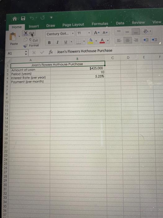
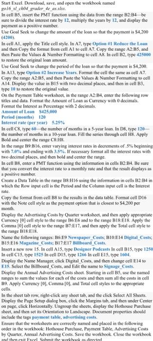
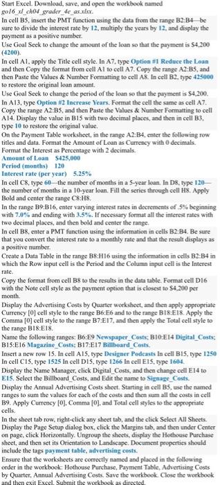
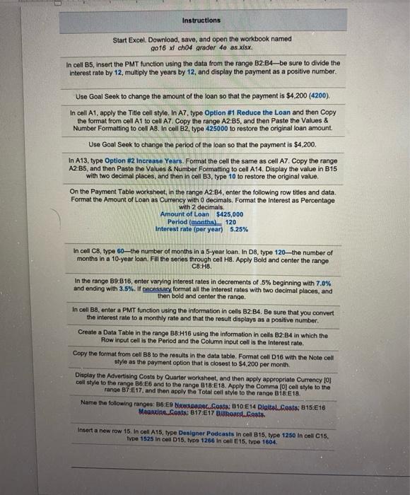
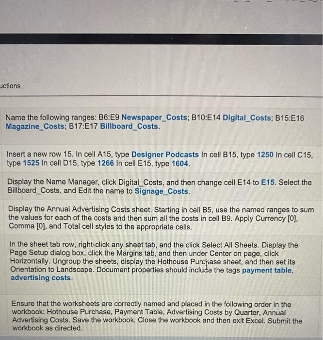
Formulas Data Review View Draw Page Layout Home Insert X ut 11 Century Got... - A- A- . Cut Format Paste 1 B A1 fx Joan's Flowers Hothouse Purchase D E A 8 1 Joan's Rowers Hothouse Purchase 2 Amount of loan 3 Period years! 4 Interest Rate (per year) 5 Payment (per month) $425,000 10 5.25% 7 B 9 10 11 12 13 14 15 16 17 18 19 20 21 22 23 24 25 26 27 28 29 30 31 32 33 34 35 36 37 Start Excel. Download, save, and open the workbook named gol6_xl_ch04 grader_4e_as.xlsx In cell B5, insert the PMT function using the data from the range B2:34 be sure to divide the interest rate by 12, multiply the years by 12, and display the payment as a positive number Use Goal Seek to change the amount of the loan so that the payment is $4,200 (4200). In cell Al, apply the Title cell style. In A7, type Option #1 Reduce the Loan and then Copy the format from cell Al to cell Az. Copy the range A2:B5, and then Paste the Values & Number Formatting to cell A&. In cell B2, type 425000 to restore the original loan amount Use Goal Seek to change the period of the loan so that the payment is $4,200 In A13, type Option #2 Increase Years, Format the cell the same as cell Az. Copy the range A2:BS, and then Paste the Values & Number Formatting to cell 114. Display the value in BIS with two decimal places, and then in cell B3. type 10 to restore the original value. On the Payment Table worksheet, in the range A2:34, enter the following row titles and data. Format the Amount of Loan as Currency with 0 decimals, Format the Interest as Percentage with 2 decimals. Amount of Loan $425,000 Period (month) 120 Interest rate (per year) 5.25% In cell C8. type 60 the number of months in a 5-year loan. In D8, type 120 the number of months in a 10-year loan, Fill the series through cell H8. Apply Bold and center the range C8H8 In the range B9:B16, enter varying interest rates in decrements of 5% beginning with 7.0% and ending with 3.5%. If necessary format all the interest rates with two decimal places, and then bold and center the range. In cell B8, enter a PMT function using the information in cells B2:B4. Be sure that you convert the interest rate to a monthly rate and that the result displays as a positive number Create a Data Table in the range B8:H16 using the information in cells B2:34 in which the Row input cell is the Period and the Column input sell is the Interest mate Copy the format from cell B8 to the results in the data table. Format cell D16 with the Note cell style as the payment option that is closest to 54.200 per month. Display the Advertising Costs by Quarter worksheet, and then apply appropriate Currency (0) cell style to the range B6: E6 and to the range BIX:E18. Apply the Comma (0) cell style to the range B2:E17, and then apply the Total cell style to the range B18E18 Name the following ranges: B6:19 Newspaper_Costs, BIO:E14 Digital Costs; B15:E16 Magazine Costs: B17:E17 Billboard Costs. Insert a new row 15. In cell Als.type Designer l'odeasts in cell B15, type 1250 In cell CIS. type 1525 In cell DIS. type 1266 In cell Els type 1604 Display the Name Manager, click Digital Costs, and then change cell E14 40 E15. Select the Billboard Costs, and Edit the name to Signage Costs Display the Annual Advertising Costs sheet Starting in cell B5, use the named ranges to sum the values for each of the costs and then sum all the costs in cell 19. Apply Currency f0. Comma (0) and Total cell styles to the appropriate cells In the sheet tab row, right-click any sheet tab, and the click Select All Sheets Display the Page Setup dialog box, click the Margins tab, and then under Center on page, click Horizontally. Ungroup the sheets, display the Hothouse Purchase sheet, and then set its Orientation to Landscape Document properties should include the tags payment table, advertising costs, Ensure that the worksheets are correctly named and placed in the following order in the workbook: Hothouse Purchase, Payment Table, Advertising Costs by Quarter, Annual Advertising Costs. Save the workbook. Close the workbook and then exit Excel Submit the werkhaak as directed Start Excel. Download, save, and open the workbook named gol6_xl_ch04 grader_de_as.xlsx In cell B5, insert the PMT function using the data from the range B2:B4 be sure to divide the interest rate by 12.multiply the years by 12, and display the payment as a positive number. Use Goal Seck to change the amount of the loan so that the payment is 54.200 (4200), In cell A1, apply the Title cell style. In A7. type Option #1 Reduce the Loan and then Copy the format from cell Al to cell A7. Copy the range A2:BS, and then Paste the Values & Number Formatting to cell A8. In cell B2. type 425000 to restore the original loan amount. Use Goal Seek to change the period of the loan so that the payment is $4.200. In A13, type Option #2 Increase Years. Format the cell the same as cell A7. Copy the range A2:B5, and then Paste the Values & Number Formatting to cell A14. Display the value in B15 with two decimal places, and then in cell B3, type 10 to restore the original value. On the Payment Table worksheet, in the range A2:B4. enter the following row titles and data. Format the Amount of Loan as Currency with decimals. Format the Interest as Percentage with 2 decimals. Amount of Loan $425.000 Period (months) 120 Interest rate (per year) 5.25% In cell C8, type 60-the number of months in a 5-year loan. In D8 type 120 the number of months in a 10-year loan. Fill the series through cell H8. Apply Bold and center the range C8:H8. In the range B9:B16, enter varying interest rates in decrements of 5% beginning with 7.0% and ending with 3.5%. If necessary format all the interest rates with two decimal places, and then bold and center the range. In cell B8, enter a PMT function using the information in cells B2-84. Be sure that you convert the interest rate to a monthly rate and that the result displays as a positive number Create a Data Table in the range B8:H16 using the information in cells B2:B4 in which the Row input cell is the Period and the Column input cell is the Interest rate. Copy the format from cell B8 to the results in the data table. Format cell D16 with the Note cell style as the payment option that is closest to $4,200 per month. Display the Advertising Costs by Quarter worksheet, and then apply appropriate Currency [0] cell style to the range B6:E6 and to the range B18:E18. Apply the Comma to cell style to the range B7:E17, and then apply the Total cell style to the range B18:18 Name the following ranges: B6:19 Newspaper_Costs BIO:E14 Digital Costs: B15:E16 Magazine Costs: B17:E17 Billboard_Costs Insert a new row 15. In cell A15, type Designer Podcasts In cell B15, type 1250 In cell C15, type 1525 In cell DIS, type 1266 In cell E13, type 1604. Display the Name Manager, click Digital Costs, and then change cell E14 to E15. Select the Billboard Costs, and Edit the name to Signage Costs. Display the Annual Advertising Costs sheet. Starting in cell B5, use the named ranges to sum the values for each of the costs and then sur all the costs in cell 19. Apply Currency [O], Comma (O), and Total cell styles to the appropriate cells In the sheet tab row, right-click any sheet tab, and the click Select All Sheets. Display the Page Setup dialog box, click the Margins tab, and then under Center on page, click Horizontally. Ungroup the sheets, display the Hothouse Purchase sheet , and then set its Orientation to Landscape. Document properties should include the tags payment table, advertising costs. Ensure that the worksheets are correctly named and placed in the following order in the workbook: Hothouse Purchase. Payment Table, Advertising Costs by Quarter, Annual Advertising Costs. Save the workbook Close the workbook and then exit Excel. Submit the workbook as directed Instructions Start Excel. Download, save, and open the workbook named go16 x ch04 grader 4e as.xlsx In cell B5, insert the PMT function using the data from the range B2B4-be sure to divide the Interest rate by 12, multiply the years by 12, and display the payment as a positive number Use Goal Seek to change the amount of the loan so that the payment is $4,200 (4200), In cell A1, apply the Title coll style. In A7, type Option #1 Reduce the Loan and then Copy the format from cell A1 to cell A7 Copy the range A2:B5, and then Paste the Values & Number Formatting to cell AB. In cell B2, type 425000 to restore the original loan amount. Use Goal Seek to change the period of the loan so that the payment is $4,200. In A13, type Option #2 Increase Years. Format the cell the same as cell A7. Copy the range A2 B5, and then Paste the Values & Number Formatting to cell A14. Display the value in B15 with two decimal places, and then in cell B3, type 10 to restore the original value. On the Payment Table worksheet, in the range A2:B4, enter the following row titles and data, Format the Amount of Loan as Currency with 0 decimals. Format the Interest as Percentage with 2 decimals Amount of Loan $425,000 Period (month) 120 Interest rate (per year) 5.25% In cell CB, type 60--the number of months in a 5-year loan. In D8, type 120--the number of months in a 10-year loan. Fill the series through cell H8. Apply Bold and center the range C8:H8 In the range B9 816, enter varying interest rates in decrements of 5% beginning with 7.0% and ending with 3.5%. If necessary format all the interest rates with two decimal places, and then bold and center the range, In cell B8, enter a PMT function using the information in cells B2 B4. Be sure that you convert the interest rate to a monthly rate and that the result displays as a positive number Create a Data Table in the range B8:H16 using the information in cells B2:B4 in which the Row Input cell is the Period and the Column input cell is the Interest rate. Copy the format from cell B8 to the results in the data table. Format cell D16 with the Note cel style as the payment option that is closest to $4,200 per month Display the Advertising Costs by Quarter worksheet, and then apply appropriate Currency 101 coll style to the range B6 E6 and to the range B18 E 18. Apply the Comma foj cell style to the range B7E17. and then apply the Total cell style to the range BIB E 18 Name the following ranges: 36 E9 NEWDARC. Sosta: 010:E 14 Rioital.foats; B15:16 Magazine Coata: B17:E17 Buhours.coats Insert a new row 15. In cell A15, type Designer Podcasts in cell B15, type 1250 In cell C15 lype 1525 in cell D15, typs 1266 In cell E15, type 1604 Instructions Start Excel. Download, save, and open the workbook named 2016 x ch04 grader 4e as x/sx. In cell B5, insert the PMT function using the data from the range B2B4-be sure to divide the Interest rate by 12, multiply the years by 12, and display the payment as a positive number. Use Goal Seek to change the amount of the loan so that the payment is $4,200 (4200), In cell A1, apply the Title cell style. In A7, type Option #1 Reduce the Loan and then Copy the format from cell A1 to cell A7 Copy the range A2:B5, and then Paste the Values & Number Formatting to cell A8. In cell B2, type 425000 to restore the original loan amount. Use Goal Seek to change the period of the loan so that the payment is $4,200. In A13, type Option #2 Increase Years. Format the cell the same as cell A7. Copy the range A2 B5, and then Paste the Values & Number Formatting to cell A14. Display the value in B15 with two decimal places, and then in cell B3, type 10 to restore the original value. On the Payment Table worksheet, in the range A2:B4, enter the following row titles and data Format the Amount of Loan as Currency with 0 decimals. Format the Interest as Percentage with 2 decimals, Amount of Loan $425,000 Period (month) 120 Interest rate (per year) 5.25% In cell CB, type 60-the number of months in a 5-year loan. In D8, type 120--the number of months in a 10-year loan. Fill the series through cell H8. Apply Bold and center the range C8:H8 In the range B9 B16, enter varying interest rates in decrements of .5% beginning with 7.0% and ending with 3.5%. If DACsay format all the interest rates with two decimal places, and then bold and center the range In cell B8, enter a PMT function using the information in cells B2 B4. Be sure that you convert the interest rate to a monthly rate and that the result displays as a positive number. Create a Data Table in the range B8:H16 using the information in cells B2:B4 in which the Row Input cell is the Period and the Column input cell is the Interest rate. Copy the format from cell B8 to the results in the data table. Format cell D16 with the Note cell style as the payment option that is closest to $4,200 per month Display the Advertising Costs by Quarter worksheet, and then apply appropriate Currency [0] coll style to the range B6 E6 and to the range B18 E 18. Apply the Comma to call style to the range B7 E17. and then apply the Total cell style to the range BIB E 18. Name the following ranges: 36 E9 NAUDARAC Siosta: 010 E14 Riotal. Roats, B15:16 Magazine Conta: B17:17 Buhours.costs. Insert a new row 15. In cell A15, type Designer Podcasts in cell B15, type 1250 in cell C15 type 1525 in cell D15, type 1266 In call E15, type 1604 uctions Name the following ranges: B6:E9 Newspaper_Costs; B10:E14 Digital_Costs; B15:E16 Magazine_Costs; B17:E17 Billboard_Costs. Insert a new row 15. In cell A15, type Designer Podcasts In cell B15, type 1250 In cell C15, type 1525 In cell D15, type 1266 In cell E15, type 1604. Display the Name Manager, click Digital_Costs, and then change cell E14 to E15. Select the Billboard_Costs, and Edit the name to Signage_Costs. Display the Annual Advertising Costs sheet. Starting in cell B5, use the named ranges to sum the values for each of the costs and then sum all the costs in cell B9. Apply Currency [O], Comma [0], and Total cell styles to the appropriate cells. In the sheet tab row, right-click any sheet tab, and the click Select All Sheets. Display the Page Setup dialog box, click the Margins tab, and then under Center on page, click Horizontally. Ungroup the sheets, display the Hothouse Purcjase sheet, and then set its Orientation to Landscape. Document properties should include the tags payment table, advertising costs. Ensure that the worksheets are correctly named and placed in the following order in the workbook: Hothouse Purchase, Payment Table, Advertising Costs by Quarter, Annual Advertising Costs. Save the workbook. Close the workbook and then exit Excel. Submit the workbook as directed. What do you mean the question is not appropriate Formulas Data Review View Draw Page Layout Home Insert X ut 11 Century Got... - A- A- . Cut Format Paste 1 B A1 fx Joan's Flowers Hothouse Purchase D E A 8 1 Joan's Rowers Hothouse Purchase 2 Amount of loan 3 Period years! 4 Interest Rate (per year) 5 Payment (per month) $425,000 10 5.25% 7 B 9 10 11 12 13 14 15 16 17 18 19 20 21 22 23 24 25 26 27 28 29 30 31 32 33 34 35 36 37 Start Excel. Download, save, and open the workbook named gol6_xl_ch04 grader_4e_as.xlsx In cell B5, insert the PMT function using the data from the range B2:34 be sure to divide the interest rate by 12, multiply the years by 12, and display the payment as a positive number Use Goal Seek to change the amount of the loan so that the payment is $4,200 (4200). In cell Al, apply the Title cell style. In A7, type Option #1 Reduce the Loan and then Copy the format from cell Al to cell Az. Copy the range A2:B5, and then Paste the Values & Number Formatting to cell A&. In cell B2, type 425000 to restore the original loan amount Use Goal Seek to change the period of the loan so that the payment is $4,200 In A13, type Option #2 Increase Years, Format the cell the same as cell Az. Copy the range A2:BS, and then Paste the Values & Number Formatting to cell 114. Display the value in BIS with two decimal places, and then in cell B3. type 10 to restore the original value. On the Payment Table worksheet, in the range A2:34, enter the following row titles and data. Format the Amount of Loan as Currency with 0 decimals, Format the Interest as Percentage with 2 decimals. Amount of Loan $425,000 Period (month) 120 Interest rate (per year) 5.25% In cell C8. type 60 the number of months in a 5-year loan. In D8, type 120 the number of months in a 10-year loan, Fill the series through cell H8. Apply Bold and center the range C8H8 In the range B9:B16, enter varying interest rates in decrements of 5% beginning with 7.0% and ending with 3.5%. If necessary format all the interest rates with two decimal places, and then bold and center the range. In cell B8, enter a PMT function using the information in cells B2:B4. Be sure that you convert the interest rate to a monthly rate and that the result displays as a positive number Create a Data Table in the range B8:H16 using the information in cells B2:34 in which the Row input cell is the Period and the Column input sell is the Interest mate Copy the format from cell B8 to the results in the data table. Format cell D16 with the Note cell style as the payment option that is closest to 54.200 per month. Display the Advertising Costs by Quarter worksheet, and then apply appropriate Currency (0) cell style to the range B6: E6 and to the range BIX:E18. Apply the Comma (0) cell style to the range B2:E17, and then apply the Total cell style to the range B18E18 Name the following ranges: B6:19 Newspaper_Costs, BIO:E14 Digital Costs; B15:E16 Magazine Costs: B17:E17 Billboard Costs. Insert a new row 15. In cell Als.type Designer l'odeasts in cell B15, type 1250 In cell CIS. type 1525 In cell DIS. type 1266 In cell Els type 1604 Display the Name Manager, click Digital Costs, and then change cell E14 40 E15. Select the Billboard Costs, and Edit the name to Signage Costs Display the Annual Advertising Costs sheet Starting in cell B5, use the named ranges to sum the values for each of the costs and then sum all the costs in cell 19. Apply Currency f0. Comma (0) and Total cell styles to the appropriate cells In the sheet tab row, right-click any sheet tab, and the click Select All Sheets Display the Page Setup dialog box, click the Margins tab, and then under Center on page, click Horizontally. Ungroup the sheets, display the Hothouse Purchase sheet, and then set its Orientation to Landscape Document properties should include the tags payment table, advertising costs, Ensure that the worksheets are correctly named and placed in the following order in the workbook: Hothouse Purchase, Payment Table, Advertising Costs by Quarter, Annual Advertising Costs. Save the workbook. Close the workbook and then exit Excel Submit the werkhaak as directed Start Excel. Download, save, and open the workbook named gol6_xl_ch04 grader_de_as.xlsx In cell B5, insert the PMT function using the data from the range B2:B4 be sure to divide the interest rate by 12.multiply the years by 12, and display the payment as a positive number. Use Goal Seck to change the amount of the loan so that the payment is 54.200 (4200), In cell A1, apply the Title cell style. In A7. type Option #1 Reduce the Loan and then Copy the format from cell Al to cell A7. Copy the range A2:BS, and then Paste the Values & Number Formatting to cell A8. In cell B2. type 425000 to restore the original loan amount. Use Goal Seek to change the period of the loan so that the payment is $4.200. In A13, type Option #2 Increase Years. Format the cell the same as cell A7. Copy the range A2:B5, and then Paste the Values & Number Formatting to cell A14. Display the value in B15 with two decimal places, and then in cell B3, type 10 to restore the original value. On the Payment Table worksheet, in the range A2:B4. enter the following row titles and data. Format the Amount of Loan as Currency with decimals. Format the Interest as Percentage with 2 decimals. Amount of Loan $425.000 Period (months) 120 Interest rate (per year) 5.25% In cell C8, type 60-the number of months in a 5-year loan. In D8 type 120 the number of months in a 10-year loan. Fill the series through cell H8. Apply Bold and center the range C8:H8. In the range B9:B16, enter varying interest rates in decrements of 5% beginning with 7.0% and ending with 3.5%. If necessary format all the interest rates with two decimal places, and then bold and center the range. In cell B8, enter a PMT function using the information in cells B2-84. Be sure that you convert the interest rate to a monthly rate and that the result displays as a positive number Create a Data Table in the range B8:H16 using the information in cells B2:B4 in which the Row input cell is the Period and the Column input cell is the Interest rate. Copy the format from cell B8 to the results in the data table. Format cell D16 with the Note cell style as the payment option that is closest to $4,200 per month. Display the Advertising Costs by Quarter worksheet, and then apply appropriate Currency [0] cell style to the range B6:E6 and to the range B18:E18. Apply the Comma to cell style to the range B7:E17, and then apply the Total cell style to the range B18:18 Name the following ranges: B6:19 Newspaper_Costs BIO:E14 Digital Costs: B15:E16 Magazine Costs: B17:E17 Billboard_Costs Insert a new row 15. In cell A15, type Designer Podcasts In cell B15, type 1250 In cell C15, type 1525 In cell DIS, type 1266 In cell E13, type 1604. Display the Name Manager, click Digital Costs, and then change cell E14 to E15. Select the Billboard Costs, and Edit the name to Signage Costs. Display the Annual Advertising Costs sheet. Starting in cell B5, use the named ranges to sum the values for each of the costs and then sur all the costs in cell 19. Apply Currency [O], Comma (O), and Total cell styles to the appropriate cells In the sheet tab row, right-click any sheet tab, and the click Select All Sheets. Display the Page Setup dialog box, click the Margins tab, and then under Center on page, click Horizontally. Ungroup the sheets, display the Hothouse Purchase sheet , and then set its Orientation to Landscape. Document properties should include the tags payment table, advertising costs. Ensure that the worksheets are correctly named and placed in the following order in the workbook: Hothouse Purchase. Payment Table, Advertising Costs by Quarter, Annual Advertising Costs. Save the workbook Close the workbook and then exit Excel. Submit the workbook as directed Instructions Start Excel. Download, save, and open the workbook named go16 x ch04 grader 4e as.xlsx In cell B5, insert the PMT function using the data from the range B2B4-be sure to divide the Interest rate by 12, multiply the years by 12, and display the payment as a positive number Use Goal Seek to change the amount of the loan so that the payment is $4,200 (4200), In cell A1, apply the Title coll style. In A7, type Option #1 Reduce the Loan and then Copy the format from cell A1 to cell A7 Copy the range A2:B5, and then Paste the Values & Number Formatting to cell AB. In cell B2, type 425000 to restore the original loan amount. Use Goal Seek to change the period of the loan so that the payment is $4,200. In A13, type Option #2 Increase Years. Format the cell the same as cell A7. Copy the range A2 B5, and then Paste the Values & Number Formatting to cell A14. Display the value in B15 with two decimal places, and then in cell B3, type 10 to restore the original value. On the Payment Table worksheet, in the range A2:B4, enter the following row titles and data, Format the Amount of Loan as Currency with 0 decimals. Format the Interest as Percentage with 2 decimals Amount of Loan $425,000 Period (month) 120 Interest rate (per year) 5.25% In cell CB, type 60--the number of months in a 5-year loan. In D8, type 120--the number of months in a 10-year loan. Fill the series through cell H8. Apply Bold and center the range C8:H8 In the range B9 816, enter varying interest rates in decrements of 5% beginning with 7.0% and ending with 3.5%. If necessary format all the interest rates with two decimal places, and then bold and center the range, In cell B8, enter a PMT function using the information in cells B2 B4. Be sure that you convert the interest rate to a monthly rate and that the result displays as a positive number Create a Data Table in the range B8:H16 using the information in cells B2:B4 in which the Row Input cell is the Period and the Column input cell is the Interest rate. Copy the format from cell B8 to the results in the data table. Format cell D16 with the Note cel style as the payment option that is closest to $4,200 per month Display the Advertising Costs by Quarter worksheet, and then apply appropriate Currency 101 coll style to the range B6 E6 and to the range B18 E 18. Apply the Comma foj cell style to the range B7E17. and then apply the Total cell style to the range BIB E 18 Name the following ranges: 36 E9 NEWDARC. Sosta: 010:E 14 Rioital.foats; B15:16 Magazine Coata: B17:E17 Buhours.coats Insert a new row 15. In cell A15, type Designer Podcasts in cell B15, type 1250 In cell C15 lype 1525 in cell D15, typs 1266 In cell E15, type 1604 Instructions Start Excel. Download, save, and open the workbook named 2016 x ch04 grader 4e as x/sx. In cell B5, insert the PMT function using the data from the range B2B4-be sure to divide the Interest rate by 12, multiply the years by 12, and display the payment as a positive number. Use Goal Seek to change the amount of the loan so that the payment is $4,200 (4200), In cell A1, apply the Title cell style. In A7, type Option #1 Reduce the Loan and then Copy the format from cell A1 to cell A7 Copy the range A2:B5, and then Paste the Values & Number Formatting to cell A8. In cell B2, type 425000 to restore the original loan amount. Use Goal Seek to change the period of the loan so that the payment is $4,200. In A13, type Option #2 Increase Years. Format the cell the same as cell A7. Copy the range A2 B5, and then Paste the Values & Number Formatting to cell A14. Display the value in B15 with two decimal places, and then in cell B3, type 10 to restore the original value. On the Payment Table worksheet, in the range A2:B4, enter the following row titles and data Format the Amount of Loan as Currency with 0 decimals. Format the Interest as Percentage with 2 decimals, Amount of Loan $425,000 Period (month) 120 Interest rate (per year) 5.25% In cell CB, type 60-the number of months in a 5-year loan. In D8, type 120--the number of months in a 10-year loan. Fill the series through cell H8. Apply Bold and center the range C8:H8 In the range B9 B16, enter varying interest rates in decrements of .5% beginning with 7.0% and ending with 3.5%. If DACsay format all the interest rates with two decimal places, and then bold and center the range In cell B8, enter a PMT function using the information in cells B2 B4. Be sure that you convert the interest rate to a monthly rate and that the result displays as a positive number. Create a Data Table in the range B8:H16 using the information in cells B2:B4 in which the Row Input cell is the Period and the Column input cell is the Interest rate. Copy the format from cell B8 to the results in the data table. Format cell D16 with the Note cell style as the payment option that is closest to $4,200 per month Display the Advertising Costs by Quarter worksheet, and then apply appropriate Currency [0] coll style to the range B6 E6 and to the range B18 E 18. Apply the Comma to call style to the range B7 E17. and then apply the Total cell style to the range BIB E 18. Name the following ranges: 36 E9 NAUDARAC Siosta: 010 E14 Riotal. Roats, B15:16 Magazine Conta: B17:17 Buhours.costs. Insert a new row 15. In cell A15, type Designer Podcasts in cell B15, type 1250 in cell C15 type 1525 in cell D15, type 1266 In call E15, type 1604 uctions Name the following ranges: B6:E9 Newspaper_Costs; B10:E14 Digital_Costs; B15:E16 Magazine_Costs; B17:E17 Billboard_Costs. Insert a new row 15. In cell A15, type Designer Podcasts In cell B15, type 1250 In cell C15, type 1525 In cell D15, type 1266 In cell E15, type 1604. Display the Name Manager, click Digital_Costs, and then change cell E14 to E15. Select the Billboard_Costs, and Edit the name to Signage_Costs. Display the Annual Advertising Costs sheet. Starting in cell B5, use the named ranges to sum the values for each of the costs and then sum all the costs in cell B9. Apply Currency [O], Comma [0], and Total cell styles to the appropriate cells. In the sheet tab row, right-click any sheet tab, and the click Select All Sheets. Display the Page Setup dialog box, click the Margins tab, and then under Center on page, click Horizontally. Ungroup the sheets, display the Hothouse Purcjase sheet, and then set its Orientation to Landscape. Document properties should include the tags payment table, advertising costs. Ensure that the worksheets are correctly named and placed in the following order in the workbook: Hothouse Purchase, Payment Table, Advertising Costs by Quarter, Annual Advertising Costs. Save the workbook. Close the workbook and then exit Excel. Submit the workbook as directed. What do you mean the question is not appropriate