GO16_XL_CH03_GRADER_3G_HW - Expenses 1.2

Project Description:

In the following project, you will edit a worksheet that will be used to summarize the operations costs for the Public Works Department.

Instructions:

For the purpose of grading the project you are required to perform the following tasks:

Step Instructions Points Possible

1 Start Excel. Download and open the file named go16_xl_ch03_grader_3g_hw.xlsx. 0.000

2 In the Expenses worksheet, calculate row totals for each Expense item in the range F5:F9. Calculate column totals for each quarter and for the Annual Total in the range B10:F10. 8.000

3 In cell G5, construct a formula to calculate the Percent of Total by dividing the Annual Total for Salaries and Benefits by the Annual Total for Totals by Quarter. Use absolute cell references as necessary, format the result in Percent Style, and then Center. Fill the formula down through cell G9. 12.000

4 Use a 3-D Pie chart to chart the Annual Total for each item. Move the chart to a new sheet and then name the sheet Annual Expenses Chart. 8.000

5 For the Chart Title, type Summary of Annual Expenses and format the chart title using WordArt Style Fill - Blue, Accent 1, Shadow. Change the Chart Title font size to 28. 6.000

6 Remove the Legend from the chart and then add Data Labels formatted so that only the Category Name and Percentage display positioned in the Center. Change the Data Labels font size to 12, and apply Bold and Italic. 8.000

7 Format the Data Series using a 3-D Format effect. Change the Top bevel and Bottom bevel to Circle. Set the Top bevel Width and Height to 50 pt and then set the Bottom bevel Width and Height to 256 pt. Change the Material to the Standard Effect Metal.

Note, the bevel name may be Round, depending on the version of Office used. 4.000

8 Display the Series Options, and then set the Angle of first slice to 125 so that the Salaries and Benefits slice is in the front of the pie. Select the Salaries and Benefits slice, and then explode the slice 10%. Change the Fill Color of the Salaries and Benefits slice to a Solid fill using Green, Accent 6, Lighter 40%. 4.000

9 Format the Chart Area by applying a Gradient fill using the Preset gradients Light Gradient Accent 4 (fourth column, first row). Format the Border of the Chart Area by adding a Solid line border using Gold, Accent 4 and a 5 pt Width. 6.000

10 Display the Page Setup dialog box, and then for this chart sheet, insert a custom footer in the left section with the file name. 4.000

11 Display the Expenses worksheet, and then by using the Quarter names and the Totals by Quarter, insert a Line with Markers chart in the worksheet. Move the chart so that its upper left corner is positioned slightly inside the upper left corner of cell A12. Drag the center-right sizing handle so that the chart extends to slightly inside the right border of column G. As the Chart Title type City of Pacifica Bay Annual Expense Summary. 10.000

12 Format the Bounds of the Vertical (Value) Axis so that the Minimum is 2100000 and the Major unit is at 50000. Format the Fill of the Chart Area with a Gradient fill by applying the Preset, Light Gradient - Accent 3 (third column, first row). Format the Plot Area with a Solid fill using White, Background 1. 10.000

13 Copy the Annual Total in cell F10 and then use Paste Special to paste Values & Number Formatting in cell B35. In cell C35, construct a formula to calculate the Projected Expenses after the forecasted increase in cell B31 is applied. Fill the formula through cell F35, and then use Format Painter to copy the formatting from cell B35 to the range C35:F35. 10.000

14 Change the Orientation of this worksheet to Landscape, and then use the Scale to Fit options to fit the Height to 1 page. From the Page Setup dialog box, center the worksheet Horizontally, and insert a custom footer in the left section with the file name. 10.000

15 Ensure that the worksheets are correctly named and placed in the following order in the workbook: Annual Expenses Chart, Expenses. Save the workbook and exit Excel. Submit the file as directed. 0.000

Total Points 100.000

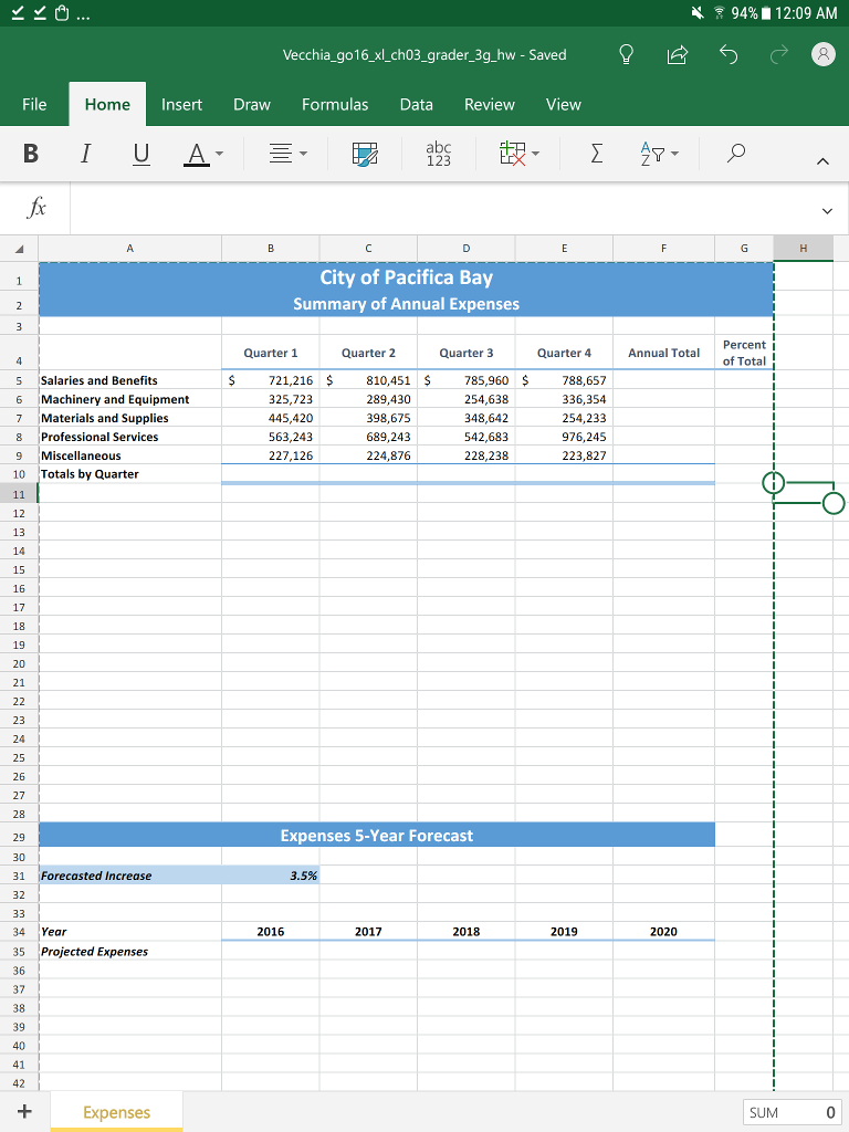
94%. 12:09 AM Vecchia.go16-xl-ch03-grader-3g.hw-Saved OBS @ File Home Insert Draw Formulas Data Review View abc 123 City of Pacifica Bay Summary of Annual Expenses Percent I of Total! Quarter 1 Quarter2 Quarter 3 Quarter 4 Annual Total 216 $ 810,451 $ S 6 7 8 9 10 Salaries and Benefits Machinery and Equipment Materials and Supplies Professional Services Miscellaneous Totals by Quarter 325,723 445,420 563,243 227,126 289,430 398,675 689,243 224,876 785,960$ 254,638 348,642 542,683 228,238 788,657 336,354 254,233 976,245 223,827 12 13 14 15 16 17 18 19 21 25 26 27 Expenses 5-Year Forecast 31 Forecasted Increase 3.5% 32 34 Year 2016 2017 2018 2019 2020 35 Projected Expenses 37 39 41 42 Expenses SUM