Good day, can you please help me. I am a working student and I don't have enough time to answer it.

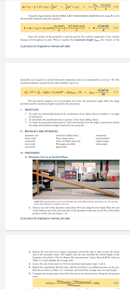
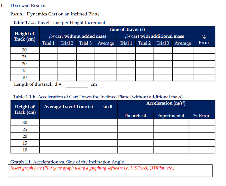
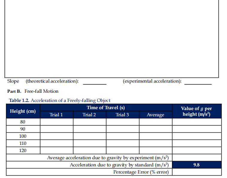
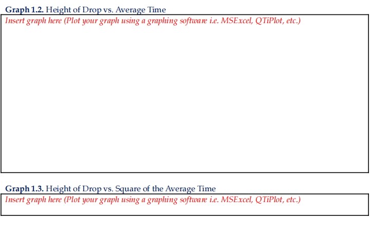
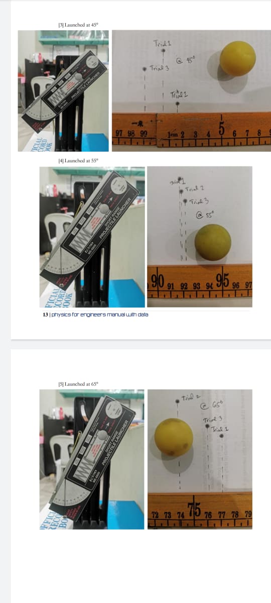
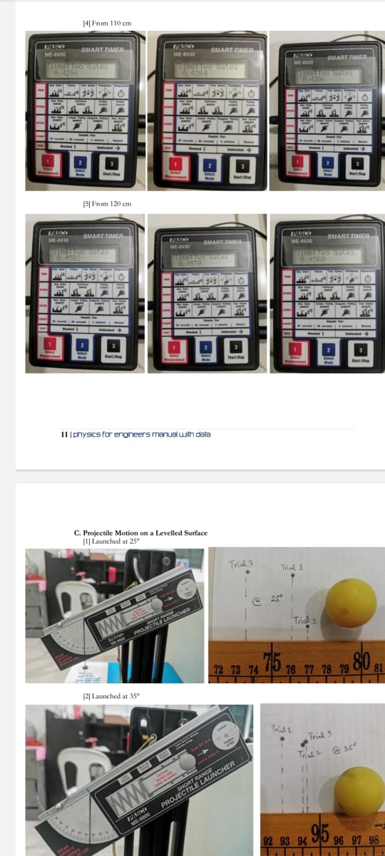
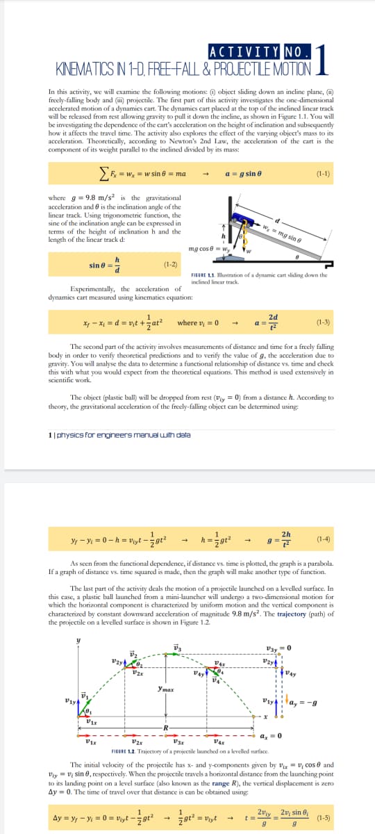
(3] Launched at 45 Trick 1 . Trial 3 -R 97 98 99 ICIAL CORD JOK [4) Launched at 55" Trial 2 SHORT RANGE PROVECHILE LAUNCHER @ 5 90 91 92 98 94 95 96 9 FICIAL CORT OOK 13 | physics for engineers manual with data [5] Launched at 65" . Trial = Trine 3 Trial 1 PROVECTILE LAUNCHER FFIC RECO 72 73 74 75 76 77 78 79position of the ball, Record in Table 1.3. Fire about three shots (three trials). 5 | physics for engineers manual with data (a) (b) FIFTIE 1.1. (a) The mini-launcher is position near the edge of a tabletop such that the launch position of the bull is homementally allyped with the table. The string indicates the angle of projection of the mini- launcher. (b) A carbon paper was placed on top of a white paper to record the landing position of the bill 5. Determined the for the average range (Rape) travelled by the plastic ball. Solve for the initial speed (v() of the ball using equation (1-6) and the maximum height (Vmax) reached by the ball using equation (1-7). 6. Repeat procedures 2-5 for the remaining angles. 7. Using a graphing software (eg. MS Excel), plot the recorded data points for range Rage vs. projection angle 0 and and draw a smooth curve through the points 8. Repeat step 7 for the recorded data points on maximum height )max vs. projection angle 6 | physics for engineers manual with data IV. DATA GATHERED FROM EXPERIMENTS A. Dynamics Cart on an Inclined Plane (Notic whether the ant aurier the social bar or not) [1] At 30 cm 12) At 25 cm[4) From 110 cm SMART TIMER ME-4920 SMART TIMER SMART TIMER 3 15] From 120 em SMART TIMER SMART RIVER ME-4130 SMART TIMER Hitapp sater 11 | physics for engineers manuel with data C. Projectile Motion on a Levelled Surface (1] Launched at 25" Trick 3 Trial 1 PROJECTRE LAUNCHER Trial 2 72 73 74 14 75 76 71 78 79 810 |2 Launched at 35% Trick ? @ 30 SHORT RANGE PROJECTILE LAUNCHER WW ME 4800 92 93 94 95 96 97 95ACTIVITY NO KINEMATICS IN 1-D. FREE FALL & PROJECTILE MOTION In this activity, we will examine the following motions: () object sliding down an incline plane, (@) freely-falling body and (ii) projectile. The first part of this activity investigates the one-dimensional accelerated motion of a dynamics cart. The dynamics cart placed at the top of the inclined linear track will be released from rest allowing gravity to pull it down the incline, as shown in Figure 1.1. You will be investigating the dependence of the cart's acceleration on the height of inclination and subsequently how it affects the travel time. The activity also explores the effect of the varying object's mass to its acceleration. Theoretically, according to Newton's 2nd Law, the acceleration of the cart is the component of its weight parallel to the inclined divided by its mass. [ =We = wsind = ma a = g sine (1-1 where g = 9.8 m/s' is the gravitational acceleration and 9 is the inclination angle of the linear track. Using trigonometric function, the sine of the inclination angle can be expressed in terms of the height of inclination h and the Vamosing length of the linear track d: my Cose = Wy sing = (1-2) FIFTH 1.1. Illustration of a dynamic cart sliding down the inclinicd lingar track. Experimentally, the acceleration of dynamics cart measured using kinematics equation: *-n= d=ut+ ;at where 1 = 0 2d (1-3) The second part of the activity involves measurements of distance and time for a freely falling body in order to verify theoretical predictions and to verify the value of g. the acceleration due to gravity. You will analyse the data to determine a functional relationship of distance vs, time and check this with what you would expect from the theoretical equations. This method is used extensively in scientific work. The object (plastic ball) will be dropped from rest (By = 0) from a distance h. According to theory, the gravitational acceleration of the freely-falling object can be determined using: 1 | physics for engineers manuel with data X - 1=0-h= but - zott - h=zgt - 2h (1-4) As seen from the functional dependence, if distance vs. time is plotted, the graph is a parabola. If a graph of distance vs. time squared is made, then the graph will make another type of function. The last part of the activity deals the motion of a projectile launched on a levelled surface, In this case, a plastic ball launched from a mini-launcher will undergo a two-dimensional motion for which the horizontal component is characterized by uniform motion and the vertical component is characterized by constant downward acceleration of magnitude 9.8 m/s". The trajectory (path) of the projectile on a levelled surface is shown in Figure 1.2 13+ =0 VAS Vzy VAY WAY y'max Piye it V1x FIfelt 1.2. Trajectory of a projectile launched on a levelled surface. The initial velocity of the projectile has x- and y-components given by V = 1, cos 0 and By = Wisin 8, respectively. When the projectile travels a horizontal distance from the launching point to its landing point on a level surface (also known as the range R), the vertical displacement is zero My = 0. The time of travel over that distance is can be obtained using: Ay = yr - y = 0 = byt -=gt# 1 = - 2v sin e (1-5)[5] At 10 cmn B, Free-fall Motion [1] From 80 cm SMART TIMER SMART TIMER ME-0930 SMART TIMER LMET TWO GATES 18591 3 9 | physics for engineers manual with data 12) From 20 cm SMART TIMER SMART TIMER SMART TIMER O (3) From 100 cm SMART TIMER SMART TIMER ME-#930 ME-0930 SMART TIMER thetwo bates 0. 4055error % Error = Valuestandard - Valueexperimental x 100% (1-8) Valuestandard 6. From the travel time measured for the cart without additional mass, use equations (1-2) and (1-1) to calculate the sine of the inclination angle (sin @) and the theoretical acceleration of the cart for each height, respectively. Record your data in Table L. I.b. 7. Calculate the experimental acceleration of the cart using equation (1-3). Compare it with the expected (theoretical) acceleration of the cart by getting the percent error using the equation (1-8) 8. Using any graphing software (e-g., MS Excel), plot a graph of the acceleration a versus sin O. Draw the best-fit straight line and calculate its slope. Determine what is this slope. Do this for both theoretical and experimental data and superimposed the two graphs. 9. Compare the slopes of the two graphs. B. Free-Fall Motion (a) (b) METH 1.4. (0 Demonstration of the experimental set-up for free-fall motion. Height use in the image in less than 30.D em. And the time-of-flight accessory is normally placed on dow door. (b) Input channels 1 and 2 on the Pason Timer device. 1. Refer to Figure 14a for the set-up of the experiment. Lay down the time-of-flight accessory on the floor. 4 | physics for engineers manuel with data 2. Position the photogate assembly at a height of 75.0 cm directly above the time-of-flight accessory. The photogate head must be vertically aligned with the time-of-flight accessory ensuring that the support stand of the Photogate assembly does not block the path. 3. Attach the connector of the photogate to the input channel 1 of the smart timer and the connector of the time-of-flight accessory to the input channel 2 of the smart timer (sec Figure 1.4b). 4. Connect the power supply of the smart timer to the outlet. Turn on the smart timer by sliding up the switch at the left side of the smart timer. 5. Using the smart timer, click the red (1) button once to select Time on the Measurement setting. Then click the blue (2) button three times to select Two-Gates Mode. This will enable the set-up to measure the time clapse of the plastic ball to hit the time-of-flight accessory. 6. Loosen the clamp screw of the photogate head to adjust the height of the sensor on the photogate matching the desired height of the ball relative to the surface of the time-of- flight accessory placed on the floor (refer to Table 1.2), then tighten it securely. 7. Position the ball your above the sensor on the photogate head without blocking the photogate beam. The built-in sensor sends signal to the device to start the measurement automatically once the beam is blocked by any object. Click on the black (3) button once to start the measurement. An . will be shown on the display indicating that device is ready for the measurement, Immediately drop the ball and record the time value displayed on the screen. Click the black (3) button once again to reset/ restart the measurement. Do this for 3 trials. 8. Then repeat steps 6 and 7 for different vertical distances and record all the data on Table 1.2. 9. For each distance, obtain an experimental value of the acceleration due to gravity using equation (1-4). 10. Calculate the average experimental value of g and compare it to the theoretical known value of g by taking its percentage error using equation (1-8). 11. Using any graphing software (eg., MS Excel), plot the recorded data points for height h vs. average time tape- On the same graph make a smooth curve of the equation. 12. Next make a plot of height h vs. square of the average time fave and determine the slope of the graph. C. Projectile Motion on a Levelled Surface 1. Position the muzzle (mouth) of the mini launcher near one end of the table so that the ball will land on the same horizontal surface (see Figure 1.5)- 2. Adjust the angle of the Mini Launcher to twenty-five (25"), Put the ball into the Mini Launcher and set it to short range (Ist) if using Type-A launcher. Type-B need not to be adjusted. Use the set range all throughout the experiment. 3. Fire a test shot to locate where the ball hits the table. At this position, tape a piece of white paper with a carbon paper on top of it to locate the landing point of the ball. 4. Fire an actual shot and measure the horizontal distance from the muzzle to the landing position of the ball. Record in Table 1.3. Fire about three shots (three trials).12) At 25 cmm 7 | physics for engineers manual with data 13) At 20 cm [4) At 15 cm 0.0 1 COM 8 | physics for engineers manual with dala 15) At 10 cmAy = 1/ - y = 0 = byt 1 + 5gta = Viyt + t=_ 2vy 21, sin 0, (1-5) g Using the trigonometric identity sin(a + #) = sin a cos # + sin / cos c, the range R can be theoretically obtained using the equation: R = Ax = Vit = (1, cos #) (-sing) 207 sing, cos B, R Uf sin 20, (1-6) 9 Since the motion of the projectile is acted by gravity, the vertical component of the velocity changes all throughout its path. When it reaches the maximum height year, the velocity of the 2 | physics for engineers manual with data projectile is just equal to its initial horizontal component (since it is momentarily at rest By = 0). The maximum distance reached by the ball vertically is given as w/y = 03 = viy - 2gay = (v, sin 8)2 - 2g(Vmax - 0) - ymar= uf sin" 0 (1-7 ) 2g The last activity requires you to investigate how does the projection angle affect the range travelled and the maximum height reached by the projection. 1. OBJECTIVES 1. To study the relationship between the acceleration of an object down an incline to its angle of inclination. 2 To determine the acceleration due to gravity of the freely falling object. 3. To study the projectile motion and to verify and describe how the angle of projection affects the range and maximum height reached by the projectile. 11. MATERIALS AND APPARATUS dynamics cart metal bar (added mass) meterstick linear track Pasco Smart timer mini-launcher stopwatch Time-of-Flight accessory carbon paper iron stand Photogate assembly white paper meterstick plastic ball III. PROCEDURES A. Dynamics Cart on an Inclined Plane I MIN FISET 1.3. Experimental set-up for the dynamics can with additional man (metal bar) on a 120 cm long Inear track inclined at a height of 30.0 cm. 1. Elevate one end of the dynamics track about 30.0 cm using the iron stand. Place the cart at the farthest end of the elevated side of the dynamics track and record this as the initial position of the cart (see Figure 1.3). 3 1 physics for engineers manual with data 2. Release the cart from rest. Using a stopwatch, record the time it takes to pass the lower end of the dynamics track. This implies that the cart travelled the whole length of the dynamics cart which is 120 cm. Repeat this measurement 3 times. Record all the values in Table 3. La and calculate the average time. 3. Lower the end of the track by 5.00 cm increment and repeat steps 1 and 2. 4. Repeat the experiment. But this time, add the metal bar as an additional mass on the cart. Record your data in Table 3.1.a. Calculate and record the average time for each height. 5. Compare the average time of travel for the cart in two situations by solving for the percent error % Error = Valuestandard - Valueexperimentall x 100% ValuestandardI. DATA AND RESULTS Part A. Dynamics Cart on an Inclined Plane Table 1.1.a. Travel Time per Height Increment Time of Travel (s) Height of Track (cm) Error 30 25 20 15 10 Table 1.1.b. Acceleration of Cart Down the Inclined Plane (without additional mass) Height of Average Travel Time (s) sin 0 Acceleration (m/s?) Track (cm) Theoretical Experimental % Error 30 25 20 15 10 Graph 1.1. Acceleration vs. Sine of the Inclination Angle Insert graph here (Plot your graph using a graphing software i.e. MSExcel, QTiPlot, etc.)Slope (theoretical acceleration): (experimental acceleration): Part B. Free-fall Motion Table 1.2. Acceleration of a Freely-falling Object Time of Travel (s) Height (cm) Value of g per Trial 1 Trial 2 Trial 3 Average height (m/s ) 80 90 100 110 120 Average acceleration due to gravity by experiment (m/s?) Acceleration due to gravity by standard (m/s?) 9.8 Percentage Error (% error)Graph 1.2. Height of Drop vs. Average Time Insert graph here (Plot your graph using a graphing software i.e. MSExcel, QTiPlot, etc.) Graph 1.3. Height of Drop vs. Square of the Average Time Insert graph here (Plot your graph using a graphing software i.e. MSExcel, QTiPlot, etc.)Part C. Projectile Motion on a Levelled Surface Table 1.3. Projectile Motion on a Level Surface Projection Initial speed Maximum Angle (") Trial 1 Average (m/s) Height (m) 25 35 45 55 65 Graph 1.4. Range vs. Projection Angle Insert graph here (Plot your graph using a graphing software i.e. MSExcel, QTiPlot, etc.) Graph 1.5. Maximum Height vs. Projection Angle Insert graph here (Plot your graph using a graphing software i.e. MSExcel, QTiPlot, etc.)II. COMPUTATIONS Insert a scanned copy/picture of your solution here with your name and signature written above the solution.III. DISCUSSION OF RESULTS Type answer here... IV. CONCLUSION Type answer here