Google colab assignment. Pls do .ipynb part in colab and word doc part in written word form. Thank you!

Lab 3.2:

Lab 4:

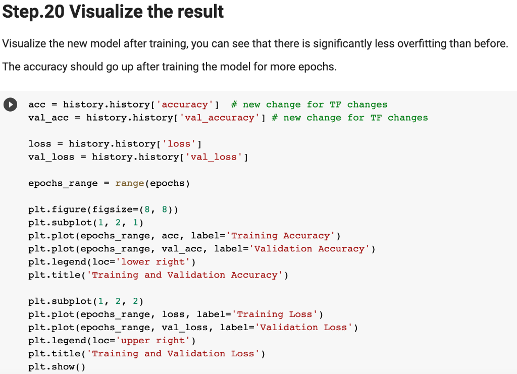
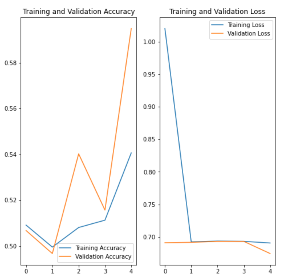
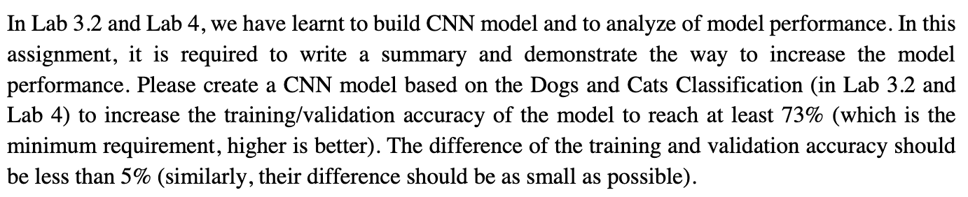
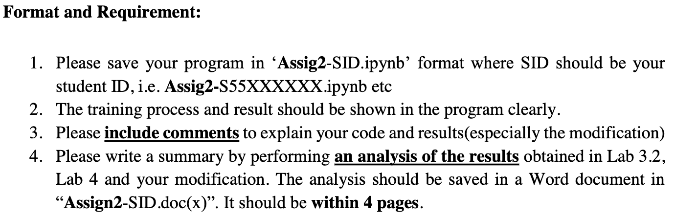
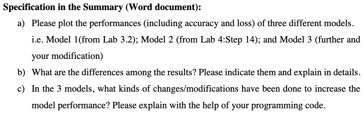
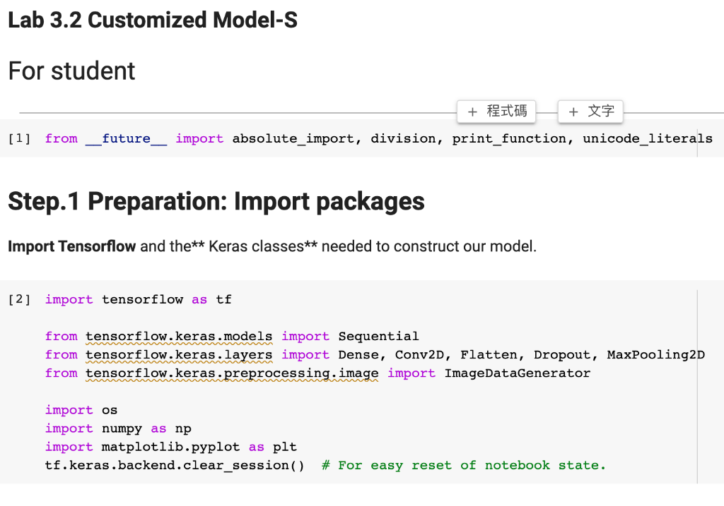
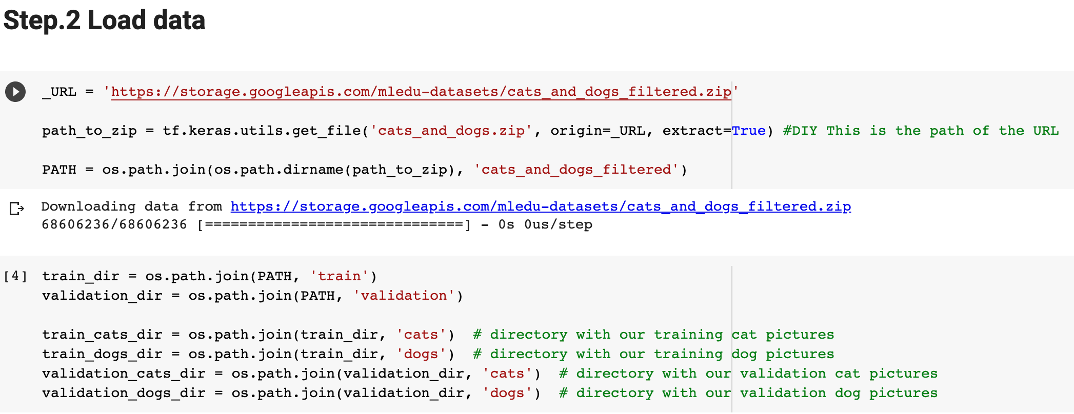
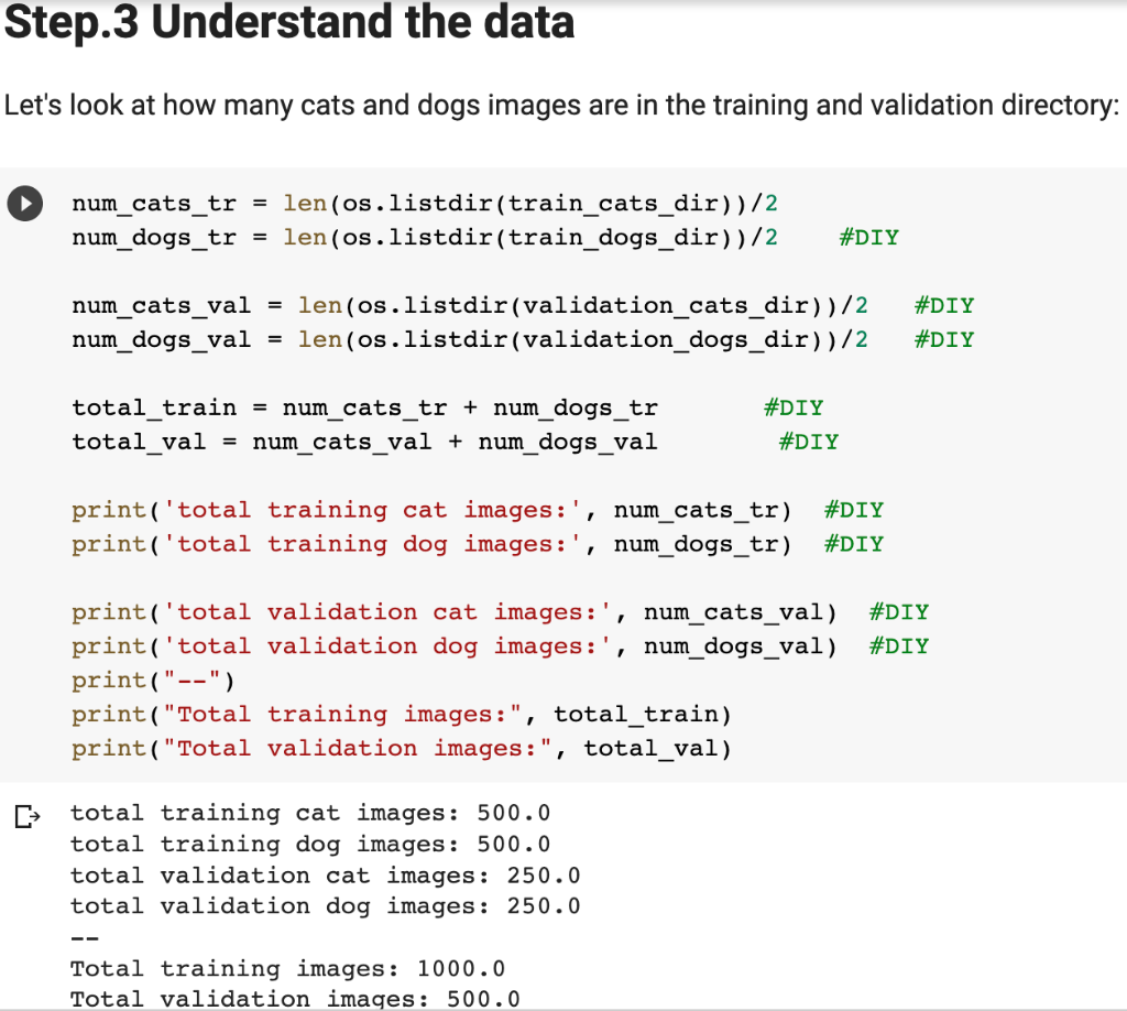
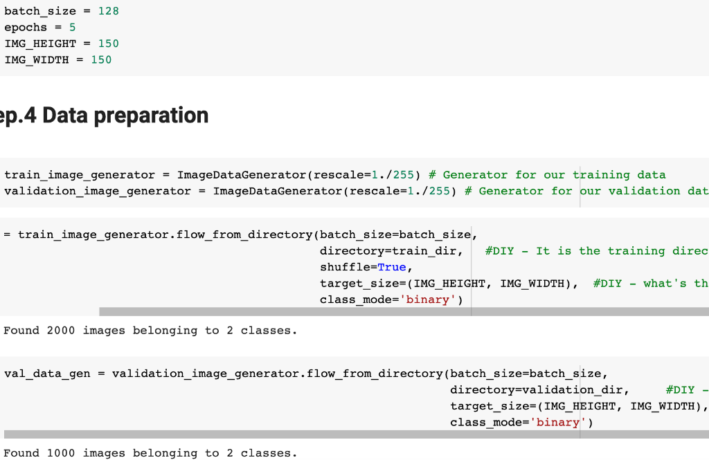
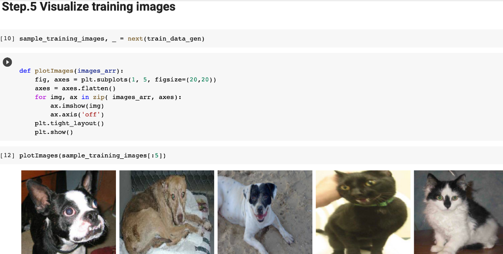
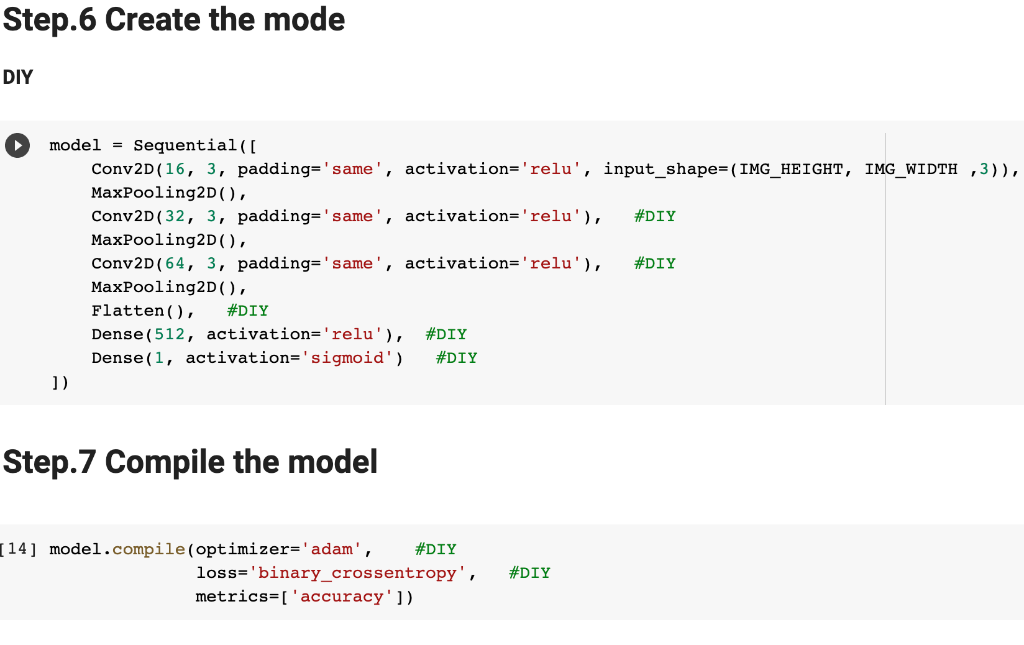
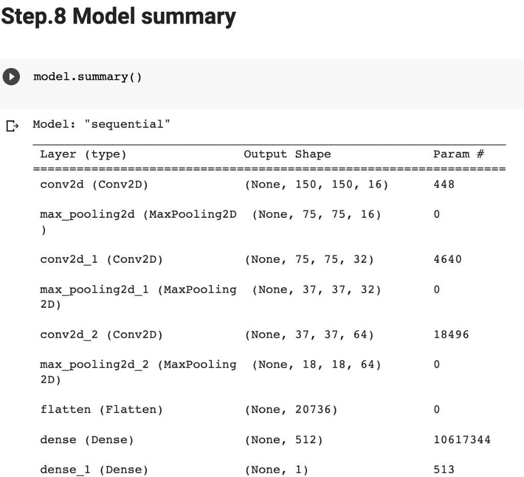
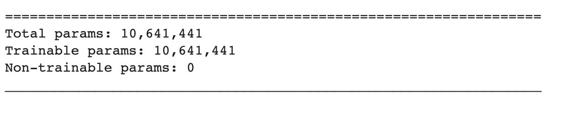
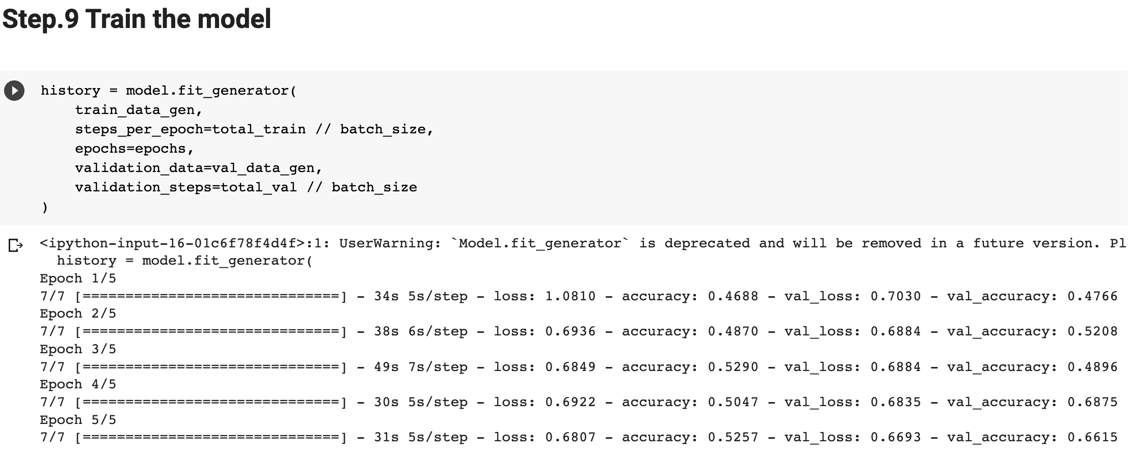
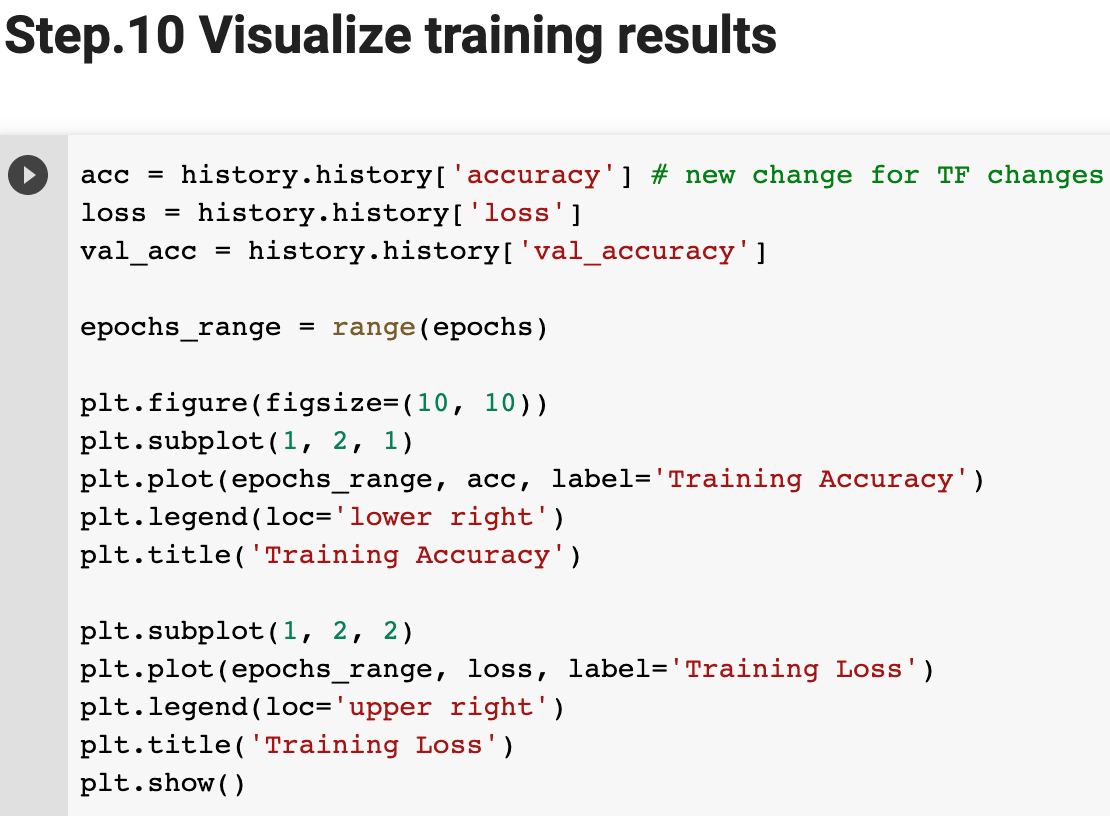
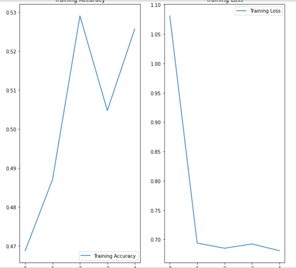
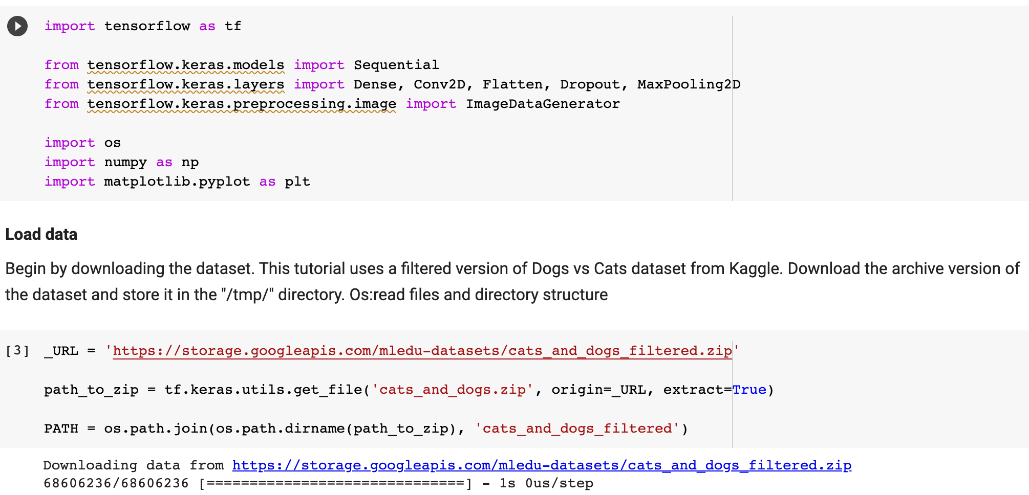
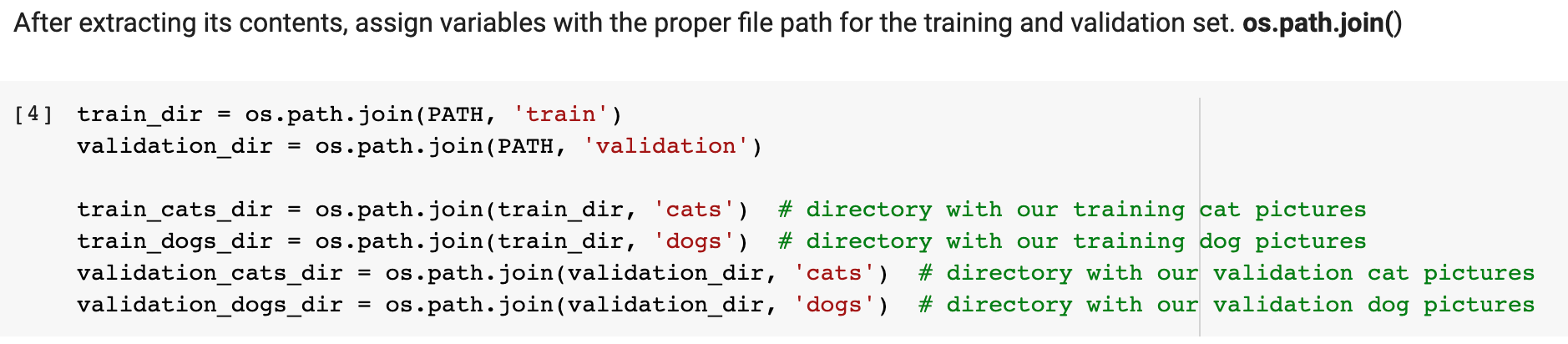
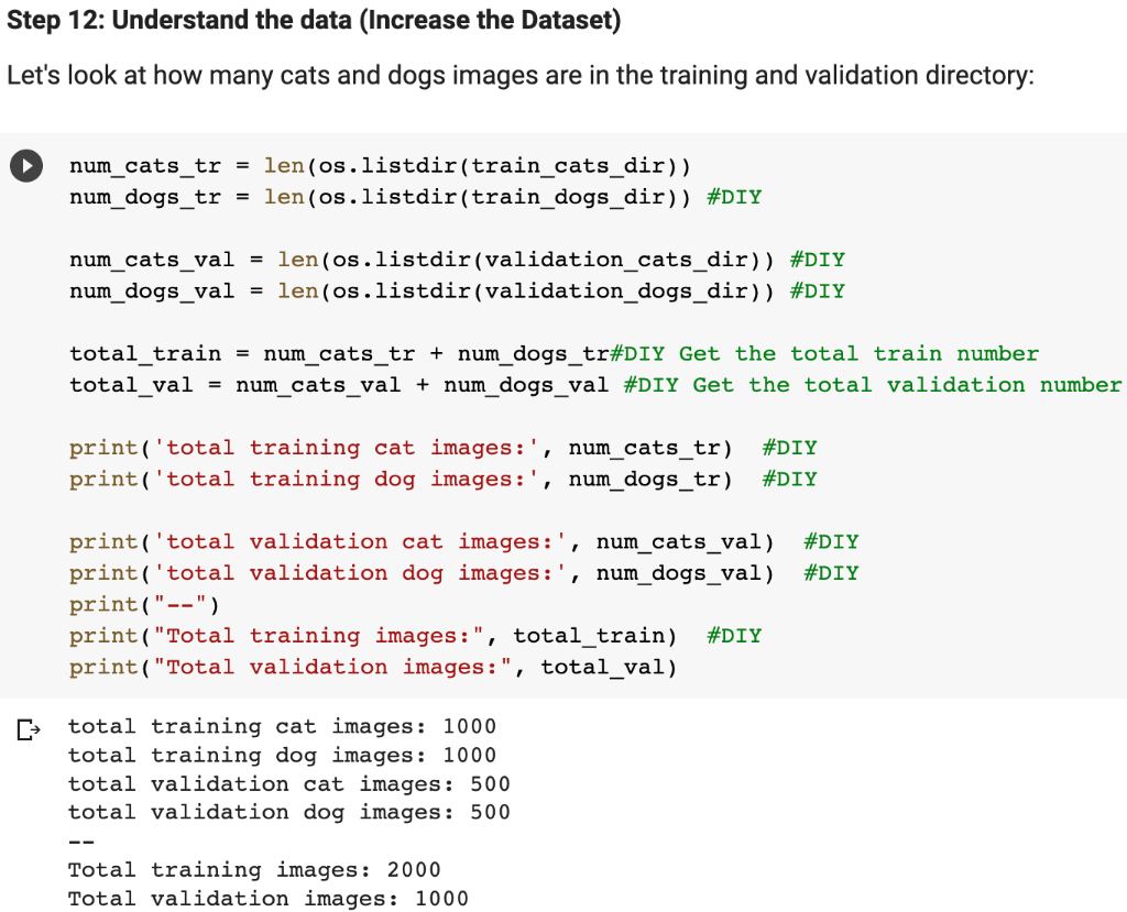
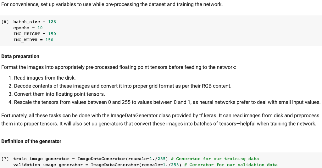
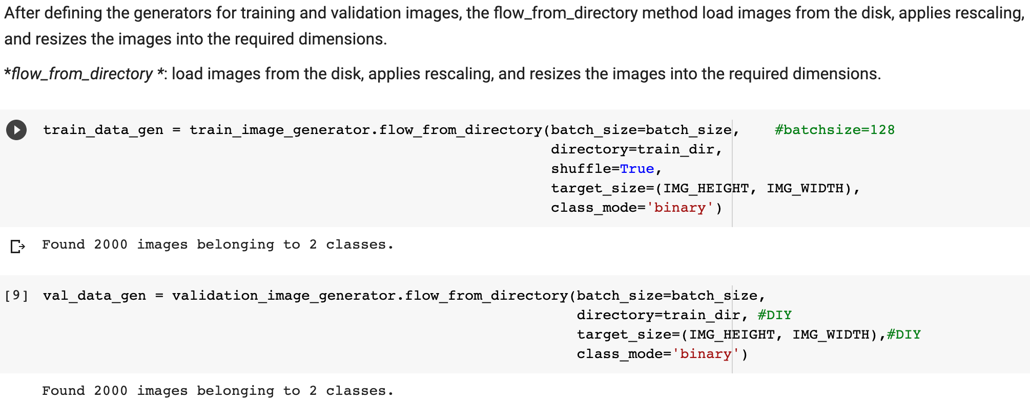
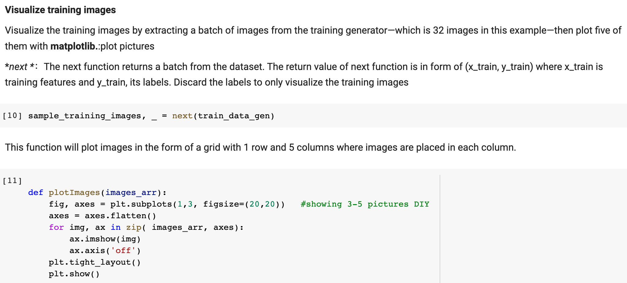
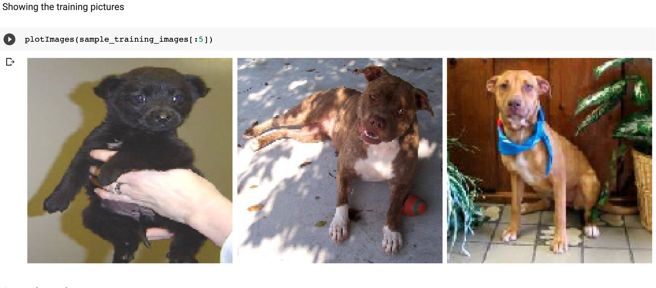
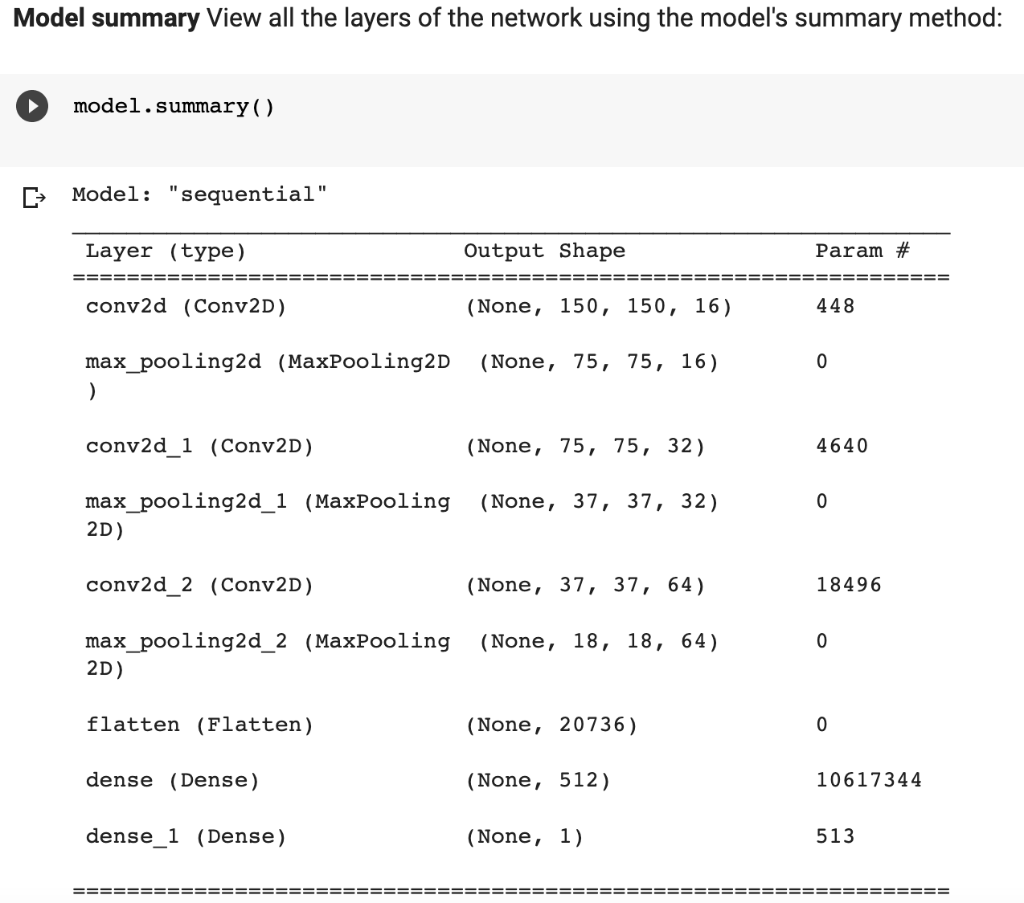
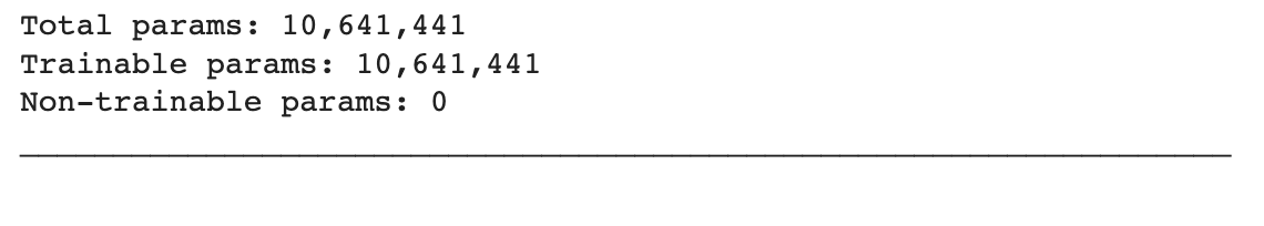
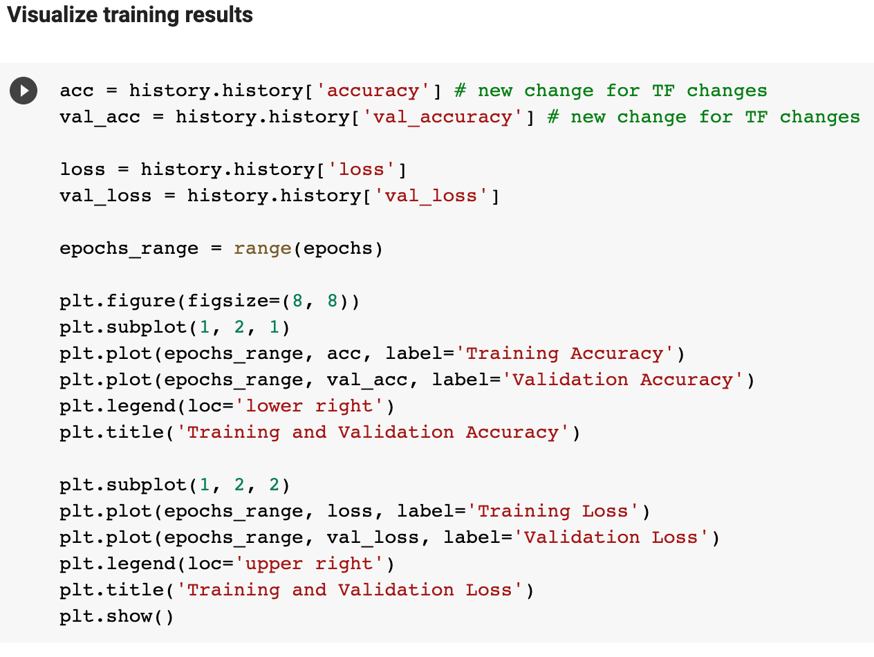
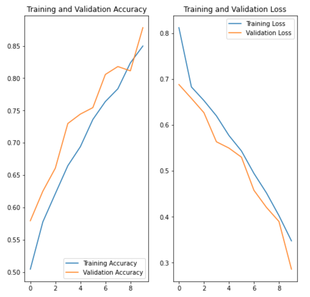
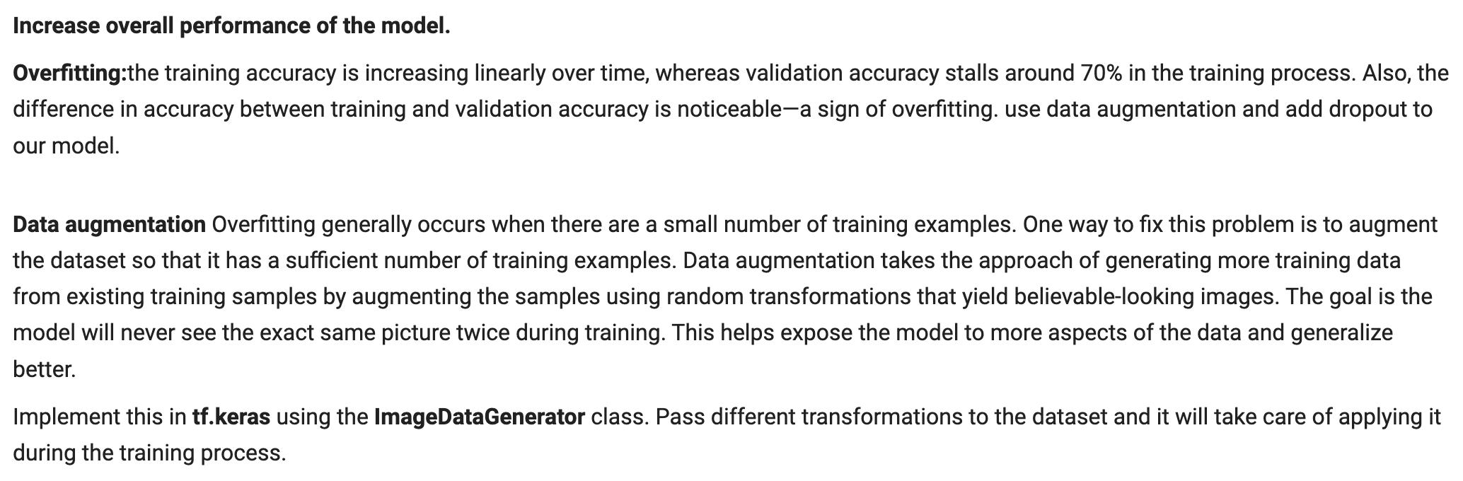
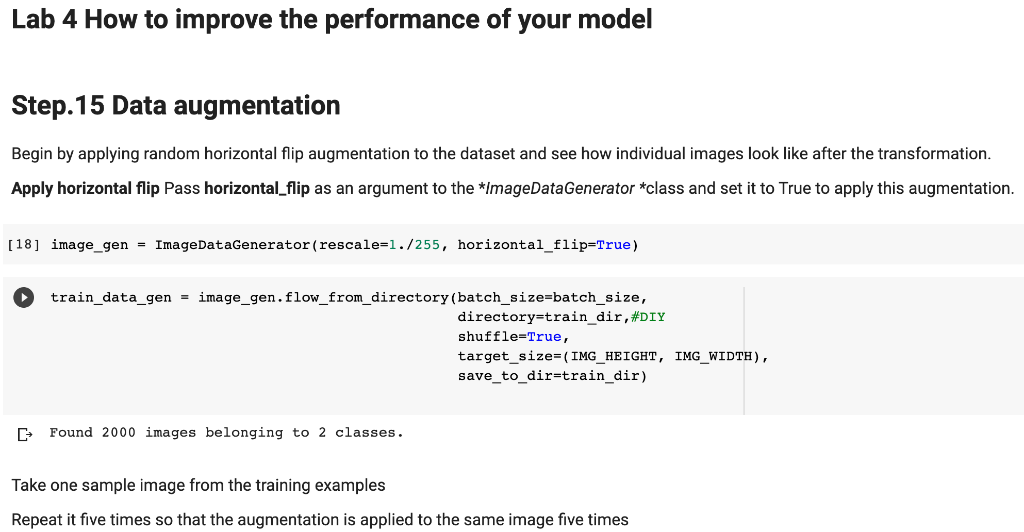
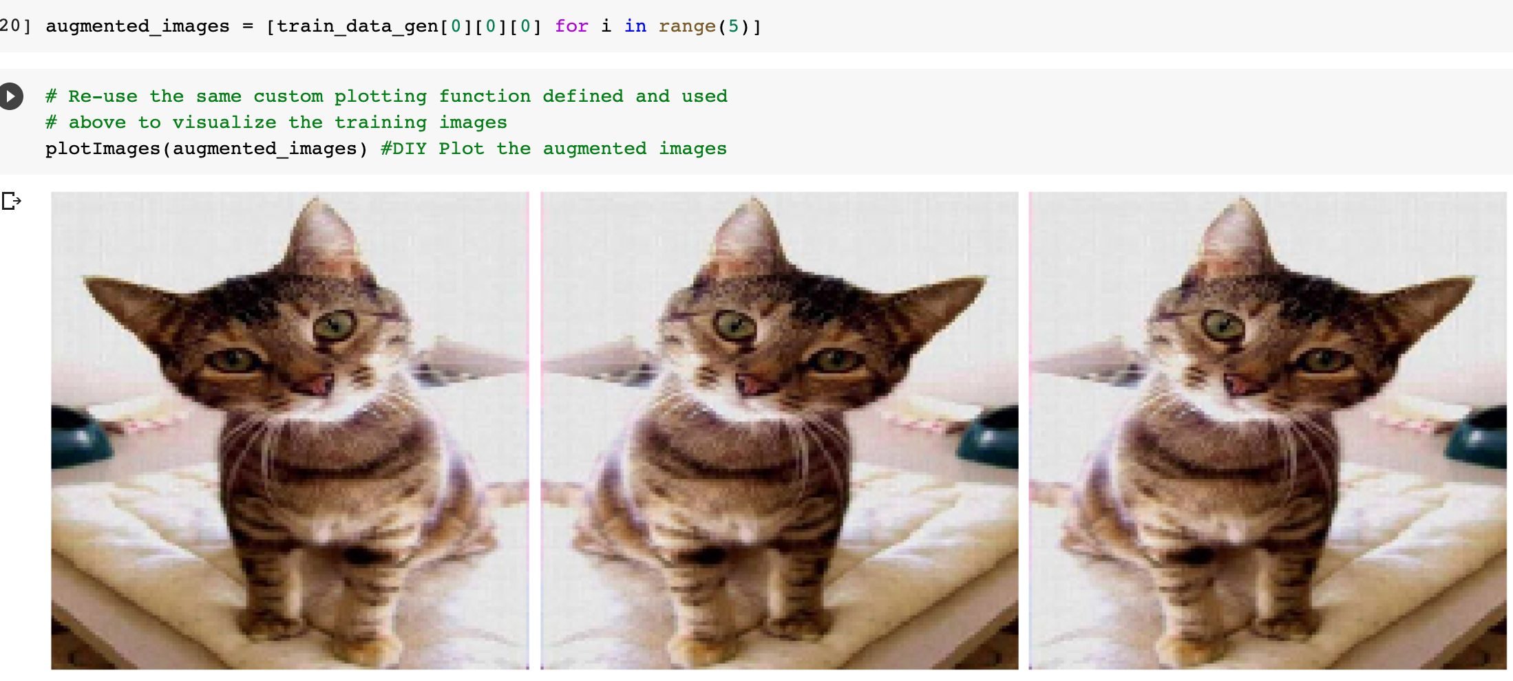
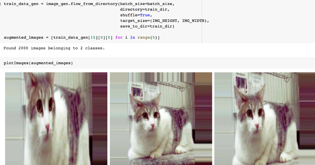
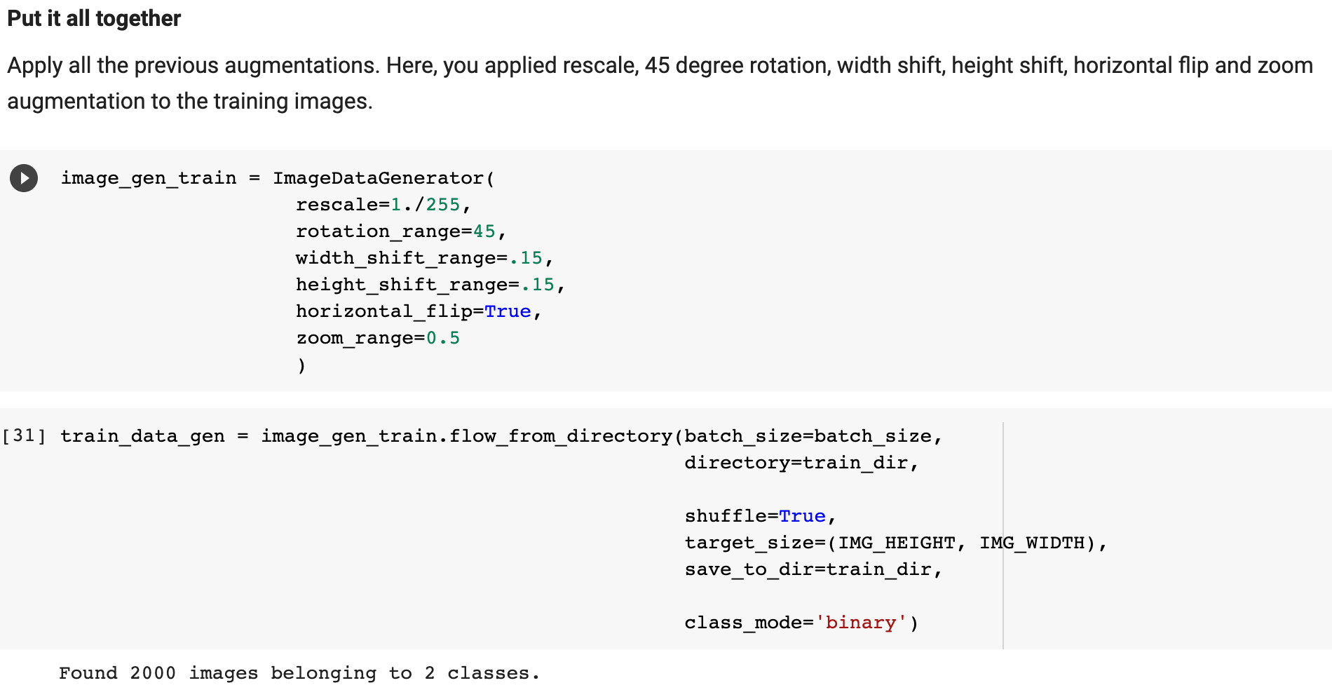
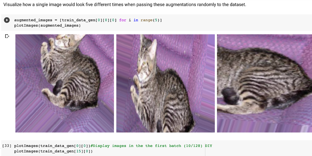
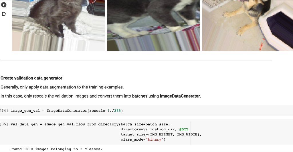
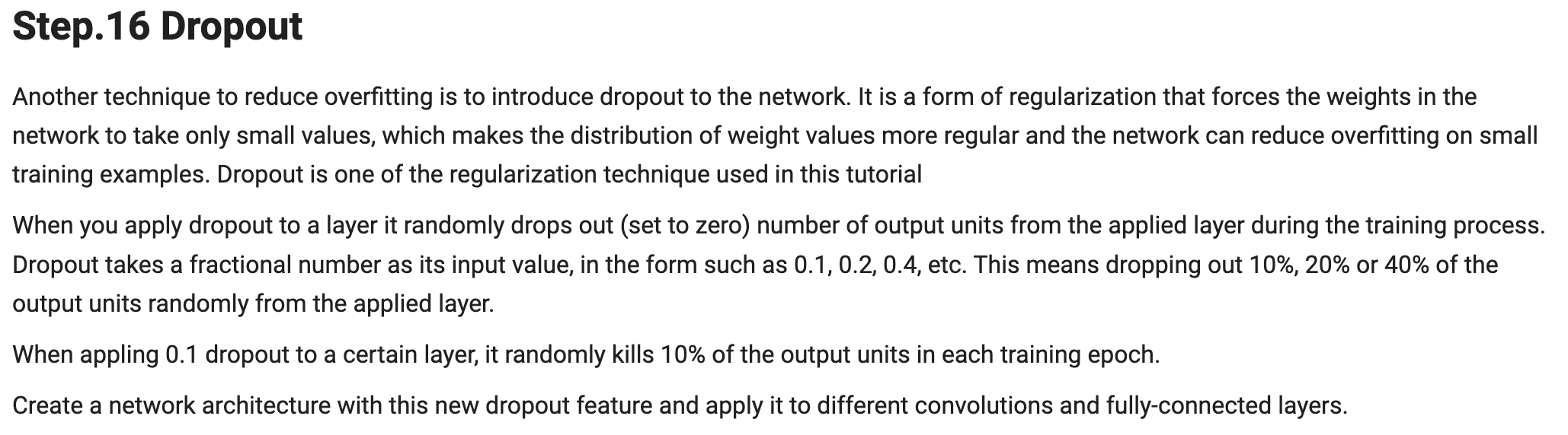
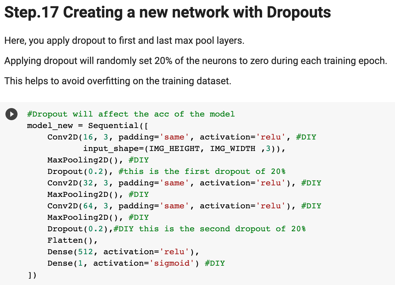
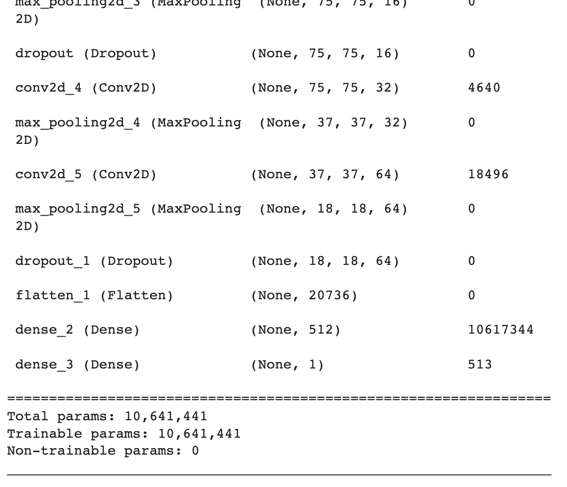
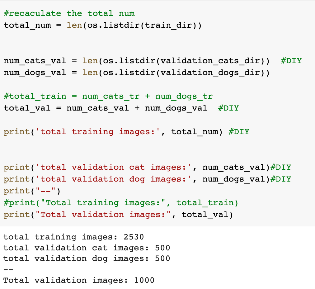
In Lab 3.2 and Lab 4, we have learnt to build CNN model and to analyze of model performance. In this assignment, it is required to write a summary and demonstrate the way to increase the model performance. Please create a CNN model based on the Dogs and Cats Classification (in Lab 3.2 and Lab 4) to increase the training/validation accuracy of the model to reach at least 73% (which is the minimum requirement, higher is better). The difference of the training and validation accuracy should be less than 5% (similarly, their difference should be as small as possible). Format and Requirement: 1. Please save your program in 'Assig2-SID.ipynb' format where SID should be your student ID, i.e. Assig2-S55XXXXXX.ipynb etc 2. The training process and result should be shown in the program clearly. 3. Please include comments to explain your code and results(especially the modification) 4. Please write a summary by performing an analysis of the results obtained in Lab 3.2, Lab 4 and your modification. The analysis should be saved in a Word document in "Assign2-SID.doc(x)". It should be within 4 pages. Specification in the Summary (Word document): a) Please plot the performances (including accuracy and loss) of three different models. i.e. Model 1(from Lab 3.2); Model 2 (from Lab 4:Step 14); and Model 3 (further and your modification) b) What are the differences among the results? Please indicate them and explain in details. c) In the 3 models, what kinds of changes/modifications have been done to increase the model performance? Please explain with the help of your programming code. Step.1 Preparation: Import packages Import Tensorflow and the Keras classes needed to construct our model. [2] import tensorflow as tf from tensorflow.keras.models import sequential from tensorflow.keras.layers import Dense, Conv2D, Flatten, Dropout, MaxPooling2D from tensorflow.keras.preprocessing.image import ImagedataGenerator import os import numpy as np import matplotlib.pyplot as plt tf.keras.backend.clear_session() \# For easy reset of notebook state. Step.2 Load data _URL = 'https://storage.googleapis.com/mledu_datasets/cats_and_dogs_filtered.zip' path_to_zip = tf.keras.utils.get_file('cats_and_dogs.zip', origin=_URL, extract=True) \#DIY This is the path of the URL PATH = os.path.join(os.path.dirname(path_to_zip), 'cats_and_dogs_filtered') C Downloading data from https://storage.googleapis.com/mledu-datasets/cats_and_dogs_filtered.zip 68606236/68606236 [=============================] - 0s 0us/step 4 ] train_dir = os.path.join(PATH, 'train') validation_dir = os.path.join(PATH, 'validation') train_cats_dir = os.path.join(train_dir, 'cats') \# directory with our training cat pictures train_dogs_dir = os.path.join(train_dir, 'dogs') \# directory with our training dog pictures validation_cats_dir = os.path.join(validation_dir, 'cats') \# directory with our validation cat pictures validation_dogs_dir = os.path.join(validation_dir, 'dogs') \# directory with our validation dog pictures s look at how many cats and dogs images are in the training and validation dire batch_size =128 epochs =5 IMG_HEIGHT =150 IMG_WIDTH =150 p.4 Data preparation Step.5 Visualize training images \[ \text { [10] sample_training_images, _ }=\text { next(train_data_gen) } \] def plotimages (images_arr): fig, axes = plt.subplots(1, 5, figsize=(20,20)) axes = axes.flatten() for img, ax in zip( images_arr, axes): ax.imshow (img) ax.axis('off') plt. tight_layout( ) plt. show () [12] plotimages (sample_training_images [:5]) model = Sequential ([ Conv2D (16,3, padding='same', activation='relu', input_shape=(IMG_HEIGHT, IMG_WIDTH ,3)), MaxPooling2D (), Conv2D (32,3, padding='same', activation='relu'), \#DIY MaxPooling2D (), Conv2D (64,3, padding='same', activation='relu'), \#DIY MaxPooling2D(), Flatten(), \#DIY Dense(512, activation='relu'), \#DIY Dense(1, activation='sigmoid') \#DIY ]) Step.7 Compile the model \( \begin{aligned}14] \text { model.compile } & \text { optimizer='adam', \#DIY } \\ & \text { loss='binary_crossentropy', \#DIY } \\ & \text { metrics=['accuracy']) }\end{aligned} \) Step.8 Model summary model. summary( () Total params: 10,641,441 Trainable params: 10,641,441 Non-trainable params: 0 Step.9 Train the model Step.10 Visualize training results acc = history.history['accuracy' ] \# new change for TF change loss = history.history['loss'] val_acc = history.history['val_accuracy'] epochs_range = range(epochs) plt.figure(figsize=( 10,10), plt.subplot(1, 2,1) plt.plot(epochs_range, acc, label='Training Accuracy') plt.legend(loc='lower right') plt.title('Training Accuracy') plt.subplot(1, 2 , 2 ) plt.plot(epochs_range, loss, label='Training Loss') plt.legend(loc='upper right') plt.title('Training Loss') plt.show() Import packages os : read files and directory structure, NumPy : convert python list to numpy array and to perform required matrix operations matplotlib.pyplot: plot the graph and display images in the training and validation data. [1] from_future_ import absolute_import, division, print_function, unicode_literals Import Tensorflow and the Keras classes needed to construct our model. import tensorflow as tf from tensorflow. keras.models import sequential from tensorflow. keras.layers import Dense, Conv2D, Flatten, Dropout, MaxPooling2D from tensorflow.keras.preprocessing.image import ImageDataGenerator import os import numpy as np import matplotlib.pyplot as plt Load data Begin by downloading the dataset. This tutorial uses a filtered version of Dogs vs Cats dataset from Kaggle. Download the archive version of the dataset and store it in the "/tmp/" directory. Os:read files and directory structure [3] _URL = 'https://storage.googleapis.com/mledu-datasets/cats_and_dogs_filtered.zip' path_to_zip = tf.keras.utils.get_file('cats_and_dogs.zip', origin=_URL, extract=True) PATH = os.path.join(os.path.dirname (path_to_zip), 'cats_and_dogs_filtered') Downloading data from https://storage.googleapis.com/mledu-datasets/cats_and_dogs_filtered.zip 68606236/68606236[===============================]1s 0us/step After extracting its contents, assign variables with the proper tile path tor the training and validation set. os.path.join() Step 12: Understand the data (Increase the Dataset) Let's look at how many cats and dogs images are in the training and validation directory: num_cats_tr = len(os.listdir(train_cats_dir)) num_dogs_tr = len(os.listdir(train_dogs_dir)) \#DIY num_cats_val = len(os.listdir(validation_cats_dir)) \#DIY num_dogs_val = len(os.listdir(validation_dogs_dir)) \#DIY total_train = num_cats_tr + num_dogs_tr\#DIY Get the total train number total_val = num_cats_val + num_dogs_val \#DIY Get the total validation number print('total training cat images:', num_cats_tr) \#DIY print('total training dog images:',num_dogs_tr) \#DIY print('total validation cat images:',num_cats_val) \#DIY print('total validation dog images:',num_dogs_val) \#DIY print("--") print("Total training images:",total_train) \#DIY print("Total validation images:",total_val) total training cat images: 1000 total training dog images: 1000 total validation cat images: 500 total validation dog images: 500 -- Total training images: 2000 Total validation images: 1000 For convenience, set up variables to use while pre-processing the dataset and training the network. [6] batch_size =128 epochs =10 IMG_HEIGHT =150 IMG_WIDTH =150 Data preparation Format the images into appropriately pre-processed floating point tensors before feeding to the network: 1. Read images from the disk. 2. Decode contents of these images and convert it into proper grid format as per their RGB content. 3. Convert them into floating point tensors. 4. Rescale the tensors from values between 0 and 255 to values between 0 and 1 , as neural networks prefer to deal with small input values Fortunately, all these tasks can be done with the ImageDataGenerator class provided by tf.keras. It can read images from disk and preprocess them into proper tensors. It will also set up generators that convert these images into batches of tensors-helpful when training the network. Definition of the generator [7] train_image_generator = ImageDatagenerator(rescale=1./255) \# Generator for our training data validation imaqe qenerator = ImaqeDataGenerator(rescale=1. /255 ) \# Generator for our validation data After defining the generators for training and validation images, the flow_from_directory method load images from the disk, applies rescaling, and resizes the images into the required dimensions. *flow_from_directory *: load images from the disk, applies rescaling, and resizes the images into the required dimensions. \[ \begin{array}{l} \text { train_data_gen = train_image_generator.flow_from_directory }(\text { batch_size=batch_size, \#batchsize=128 } \\ \text { directory=train_dir, } \\ \text { shuffle=True, } \\ \text { target_size=(IMG_HEIGHT, IMG_WIDTH ), } \\ \text { class_mode= 'binary') } \\ \end{array} \] Found 2000 images belonging to 2 classes. \[ \begin{array}{r} \text { [9] val_data_gen }=\text { validation_image_generator.flow_from_directory(batch_size=batch_size, } \\ \text { directory=train_dir, \#DIY } \\ \text { target_size=(IMG_HEIGHT, IMG_WIDTH),\#DIY } \\ \text { class_mode='binary') } \end{array} \] Found 2000 images belonging to 2classes. Visualize training images Visualize the training images by extracting a batch of images from the training generator-which is 32 images in this example-then plot five of them with matplotlib.:plot pictures *next *: The next function returns a batch from the dataset. The return value of next function is in form of (x_train, y_train) where xtrain is training features and y_train, its labels. Discard the labels to only visualize the training images [10] sample_training_images, _= next(train_data_gen) This function will plot images in the form of a grid with 1 row and 5 columns where images are placed in each column. [11] def plotimages(images_arr): fig, axes = plt.subplots(1,3, figsize=(20,20)) \#showing 3-5 pictures DIY axes = axes.flatten() for img, ax in zip( images_arr, axes): ax.imshow(img) ax.axis('off') plt.tight_layout () plt.show () Showing the training pictures \[ \text { plotimages (sample_training_images }[: 5] \text { ) } \] Model summary View all the layers of the network using the model's summary method: model. summary () Total params: 10,641,441 Trainable params: 10,641,441 Non-trainable params: 0 Train the model Use the fit_generator method of the ImageDataGenerator class to train the network. Visualize training results acc = history.history['accuracy'] \# new change for TF changes val_acc = history.history['val_accuracy'] \# new change for TF changes loss = history.history['loss'] val_loss = history.history['val_loss'] epochs_range = range(epochs) plt.figure(figsize=(8, 8)) plt.subplot(1,2, 1) plt.plot(epochs_range, acc, label='Training Accuracy') plt.plot(epochs_range, val_acc, label='Validation Accuracy') plt.legend(loc='lower right') plt.title('Training and Validation Accuracy') plt.subplot(1,2,2) plt.plot(epochs_range, loss, label='Training Loss') plt.plot(epochs_range, val_loss, label='Validation Loss') plt.legend(loc='upper right') plt.title('Training and Validation Loss') plt.show() Training and Validation Accuracy Training and Validation Loss Increase overall performance of the model. Overfitting:the training accuracy is increasing linearly over time, whereas validation accuracy stalls around 70% in the training process. Also, the difference in accuracy between training and validation accuracy is noticeable-a sign of overfitting. use data augmentation and add dropout to our model. Data augmentation Overfitting generally occurs when there are a small number of training examples. One way to fix this problem is to augment the dataset so that it has a sufficient number of training examples. Data augmentation takes the approach of generating more training data from existing training samples by augmenting the samples using random transformations that yield believable-looking images. The goal is the model will never see the exact same picture twice during training. This helps expose the model to more aspects of the data and generalize better. Implement this in tf.keras using the ImageDataGenerator class. Pass different transformations to the dataset and it will take care of applying it during the training process. Lab 4 How to improve the performance of your model Step. 15 Data augmentation Begin by applying random horizontal flip augmentation to the dataset and see how individual images look like after the transformation. Apply horizontal flip Pass horizontal_flip as an argument to the *imageDataGenerator *class and set it to True to apply this augmentation. [18] image_gen = ImageDataGenerator (rescale=1./255, horizontal_flip=True) \[ \begin{aligned} \text { train_data_gen = image_gen.flow_from_directory } & \text { batch_size=batch_size, } \\ & \text { directory=train_dir,\#DIY } \\ & \text { shuffle=True, } \\ & \text { target_size=(IMG_HEIGHT, IMG_WIDTH), } \\ & \text { save_to_dir=train_dir) } \end{aligned} \] Found 2000 images belonging to 2 classes. Take one sample image from the training examples Repeat it five times so that the augmentation is applied to the same image five times \# Re-use the same custom plotting function defined and used \# above to visualize the training images plotimages(augmented_images) \#DIY Plot the augmented images Randomly rotate the image Let's take a look at a different augmentation called rotation and apply 45 degrees of rotation randomly to the training examples. [22] image_gen = Imagedatagenerator (rescale=1./255, rotation_range=45) \#save the generated images to the file 'generated images' train_data_gen = image_gen.flow_from_directory (batch_size=batch_size, directory=train_dir, shuffle=True, target_size= ( IMG_HEIGHT, IMG_WIDTH ), save_to_dir=' /content/generated_images') augmented_images =[ train_data_gen [0][0][0] for i in range(5)] L Found 2000 images belonging to 2 classes. [25] \#save the generated images to train directory directory=train_dir,\#DIY shuffle=True, target_size =( IMG_HEIGHT, IMG_WIDTH ), save_to_dir=train_dir) augmented_images = [train_data_gen[0][0][0] for i in range(5)] Found 2000 images belonging to 2 classes. plotimages (augmented_images) Apply zoom augmentation Apply a zoom augmentation to the dataset to zoom images up to 50% randomly. [27] image_gen = ImageDatagenerator ( rescale =1./255, zoom_range =0.5) Put it all together Apply all the previous augmentations. Here, you applied rescale, 45 degree rotation, width shift, height shift, horizontal flip and zoom augmentation to the training images. directory=train_dir, shuffle=True, target_size=(IMG_HEIGHT, IMG_WIDTH), save_to_dir=train_dir, class_mode = 'binary') Found 2000 images belonging to 2 classes. Visualize how a single image would look five different times when passing these augmentations randomly to the dataset. augmented_images =[train_data_gen[0][0][0]fori in range(5)] plotimages (augmented_images ) I [33] plotImages(train_data_gen[0][0])\#Display images in the the first batch (10/128) DIY plotImages(train_data_gen[15][0]) Create validation data generator Generally, only apply data augmentation to the training examples. In this case, only rescale the validation images and convert them into batches using ImageDataGenerator. [34] image_gen_val = ImageDataGenerator (rescale=1./255) Found 1000 images belonging to 2classes. Another technique to reduce overfitting is to introduce dropout to the network. It is a form of regularization that forces the weights in the network to take only small values, which makes the distribution of weight values more regular and the network can reduce overfitting on small training examples. Dropout is one of the regularization technique used in this tutorial When you apply dropout to a layer it randomly drops out (set to zero) number of output units from the applied layer during the training process. Dropout takes a fractional number as its input value, in the form such as 0.1,0.2,0.4, etc. This means dropping out 10%,20% or 40% of the output units randomly from the applied layer. When appling 0.1 dropout to a certain layer, it randomly kills 10% of the output units in each training epoch. Create a network architecture with this new dropout feature and apply it to different convolutions and fully-connected layers. Step.17 Creating a new network with Dropouts lere, you apply dropout to first and last max pool layers. pplying dropout will randomly set 20% of the neurons to zero during each training epoch. his helps to avoid overfitting on the training dataset. \#Dropout will affect the acc of the model model_new = Sequential( [ Conv2D(16,3, padding='same', activation='relu', \#DIY input_shape=(IMG_HEIGHT, IMG_WIDTH,3)), MaxPooling2D(), \#DIY Dropout(0.2), \#this is the first dropout of 20% Conv2D(32,3, padding='same', activation='relu'), \#DIY MaxPooling2D (), \#DIY Conv2D(64, 3, padding='same', activation='relu'), \#DIY MaxPooling2D(), \#DIY Dropout(0.2),\#DIY this is the second dropout of 20% Flatten(), Dense(512, activation='relu'), Dense(1, activation='sigmoid') \#DIY ]) Step.18 Compile the model After introducing dropouts to the network, compile the model and view the layers summary. 2D) \#recaculate the total num total_num = len(os.listdir(train_dir)) num_cats_val = len(os.listdir(validation_cats_dir)) \#DIr num_dogs_val = len(os.listdir(validation_dogs_dir)) \#total_train = num_cats_tr + num_dogs_tr total_val = num_cats_val + num_dogs_val \#DIY print('total training images:',total_num) \#DIY print('total validation cat images:',num_cats_val)\#DIY print('total validation dog images:',num_dogs_val)\#DIY print("--") \#print("Total training images:", total_train) print("Total validation images:", total_val) total training images: 2530 total validation cat images: 500 total validation dog images: 500 -- Total validation images: 1000 _data_gen, Step.20 Visualize the result isualize the new model after training, you can see that there is significantly less overfitting than befo he accuracy should go up after training the model for more epochs. acc = history.history['accuracy'] \# new change for TF changes val_acc = history.history['val_accuracy'] \# new change for TF changes loss = history.history['loss'] val_loss = history.history['val_loss'] epochs_range = range(epochs) plt.figure(figsize=(8, 8)) plt.subplot(1, 2, 1 ) plt.plot(epochs_range, acc, label='Training Accuracy') plt.plot(epochs_range, val_acc, label='Validation Accuracy') plt.legend(loc='lower right') plt.title('Training and Validation Accuracy') plt.subplot(1, 2,2 ) plt.plot(epochs_range, loss, label='Training Loss') plt.plot(epochs_range, val_loss, label='Validation Loss') plt.legend(loc='upper right') plt.title('Training and Validation Loss') plt.show() Training and Validation Accuracy Training and Validation Loss