Group Project
simple linear regression analysis
multiple linear regression analysis
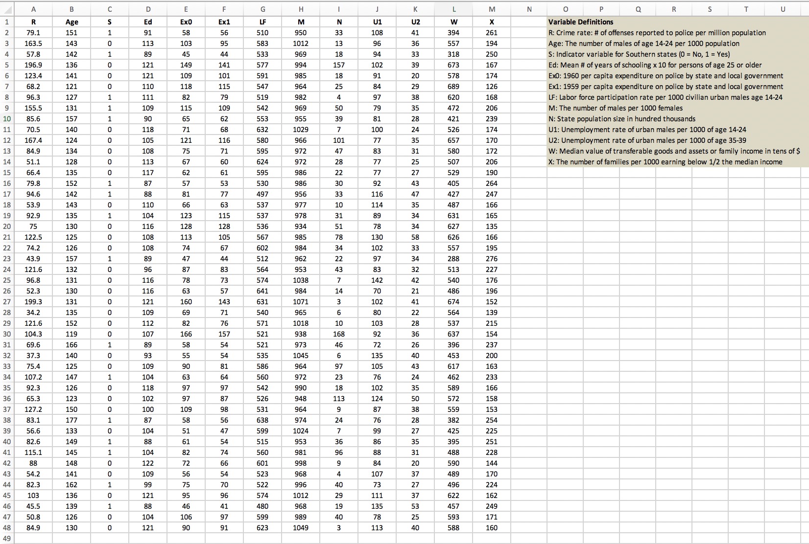
N P Q S T U G H J K L M 0 R A B C D E F Ed Exo Ex1 LF M N U1 U2 W X Variable Definitions R Age 56 510 950 33 108 41 394 261 R: Crime rate: # of offenses reported to police per million population 79.1 151 91 58 103 95 583 1012 13 96 36 557 194 Age: The number of males of age 14-24 per 1000 population 163.5 143 113 18 94 33 318 250 S: Indicator variable for Southern states (0 = No, 1 = Yes) OUT AWNI 57.8 142 89 45 44 533 969 994 157 102 39 673 167 Ed: Mean # of years of schooling x 10 for persons of age 25 or older 196.9 136 121 149 141 577 578 174 EXO: 1960 per capita expenditure on police by state and local government 123.4 141 121 109 101 591 985 18 91 20 84 29 689 126 Ex1: 1959 per capita expenditure on police by state and local government 68.2 121 110 118 115 547 964 25 82 79 519 982 97 38 620 168 LF: Labor force participation rate per 1000 civilian urban males age 14-24 96.3 127 111 969 50 79 35 472 206 M: The number of males per 1000 females 542 155.5 131 109 115 109 553 955 39 81 28 421 239 N: State population size in hundred thousands 10 85.6 157 30 65 62 118 71 68 632 1029 100 24 526 174 U1: Unemployment rate of urban males per 1000 of age 14-24 70.5 140 35 657 170 U2: Unemployment rate of urban males per 1000 of age 35-39 167.4 124 105 121 116 580 966 101 77 75 71 595 972 47 83 31 580 172 W: Median value of transferable goods and assets or family income in tens of $ 13 84.9 134 108 206 X: The number of families per 1000 earning below 1/2 the median income O O 507 14 51.1 128 113 67 60 624 972 28 77 25 77 27 529 190 15 66.4 135 0 117 62 61 595 986 22 264 16 79.8 152 87 57 53 530 986 30 92 43 405 956 33 116 47 427 247 17 94.6 142 88 81 77 497 487 166 18 53.9 143 110 66 63 537 977 10 114 35 135 104 123 115 537 978 31 89 34 631 165 92.9 OOHOH 19 128 536 934 51 78 34 627 135 20 75 130 116 128 985 78 130 58 626 166 122.5 125 108 113 105 567 IN 74.2 126 108 74 67 602 984 34 102 33 557 195 44 512 962 22 97 34 288 276 43.9 157 O HO 89 47 121.6 132 96 87 83 564 953 43 83 32 513 227 24 78 73 574 1038 142 42 540 176 25 96.8 131 116 63 57 641 984 70 21 486 196 26 52.3 130 116 O W A V 152 131 121 160 143 674 631 1071 102 41 27 199.3 135 109 69 71 540 965 80 22 564 139 28 34.2 76 571 1018 10 103 28 537 215 29 121.6 152 112 82 938 168 92 36 637 154 30 104.3 119 107 166 157 521 166 89 58 54 521 973 46 72 26 396 237 31 69.6 O O HO 32 140 93 55 54 535 1045 135 40 453 200 37.3 33 75.4 125 109 90 81 586 964 97 105 43 617 163 24 462 233 34 107.2 147 104 63 64 560 972 23 76 35 589 166 35 92.3 126 118 97 97 542 990 18 102 36 65.3 123 OOO 102 97 87 526 948 113 124 50 572 158 150 100 109 98 531 964 9 87 38 559 153 37 127.2 24 76 28 382 254 638 974 38 83.1 177 37 58 56 425 225 39 56.6 133 104 51 47 599 1024 99 27 149 38 61 54 515 953 36 86 35 395 251 40 82.6 145 104 82 74 560 981 96 88 31 488 228 115.1 72 66 601 998 84 20 590 144 88 148 122 170 43 54.2 141 OH OHOOHKO 109 56 54 523 968 107 37 489 44 32.3 162 99 75 70 522 996 10 73 27 496 224 121 95 96 574 1012 29 111 37 622 162 45 103 136 46 249 46 45.5 139 88 41 480 968 19 135 53 457 47 50.8 126 104 106 97 599 989 40 78 25 593 171 91 623 1049 3 113 40 58 8 160 48 84.9 130 121 90Ct) Simple Linear Regression Analysis (SLR) Perform a SLR with your dependent variable and the independent quantitative variable having the highest correlation with your dependent variable. Use your scatter diagram from :5): Place this chart on the same worksheet as where the estimated regression equation is located. Add a trend line and the estimated regression equation to the chart. Copy it to your Word document and comment on the following items: 1. What does it tell you about the relationship between the two variables? 2. State the population regression model to be estimated. 3. Describe the goodness of fit of the estimated regression line. 4. State the least-squares estimates of the slope and the intercept. 5. Give practical meanings (interpret the values) to the estimated slope and intercept. Multiple Linear Regression Analysis (MLR) Perform two different MLRs of your dependent variable against a selection of your independent variables, and use the Partial Ftest to compare the two models. On the basis of this test, which of the two models is the preferred one? Comment on why this is the preferred model. Given the correlations among the independent variables that you found earlier, are there any reasons to believe that we may have substantial multicollinearity? What does this mean? Comment on this in your Word document and, if necessary, undertake a remedy