Harvard University FIN 900 Assignment #4 Case Study:

Time Series Forecasting and Centered Moving Averages

(LETS GOOO CHEGG LETS GO) Please show correct excel ouput for a thumbs up!

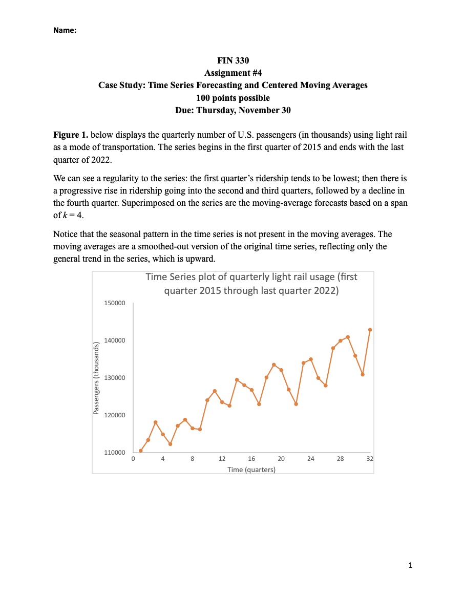
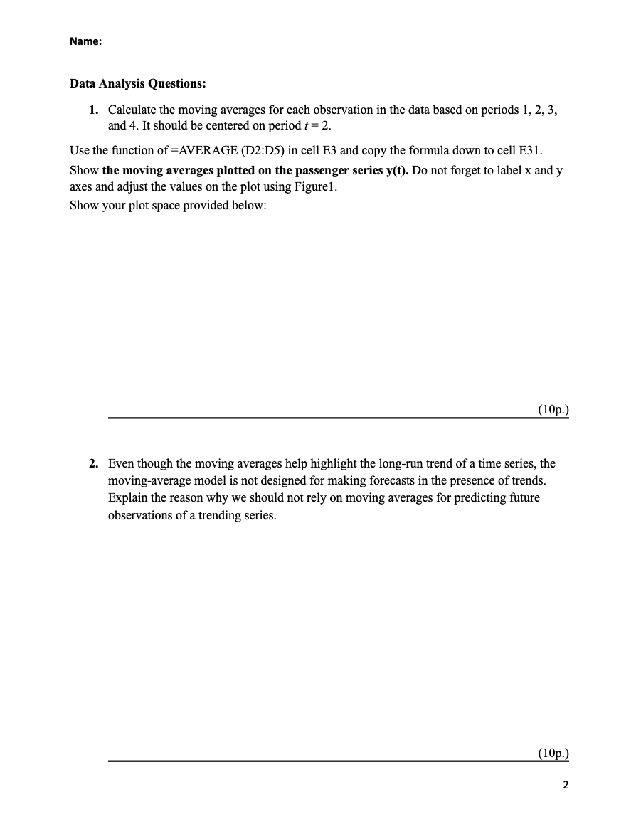
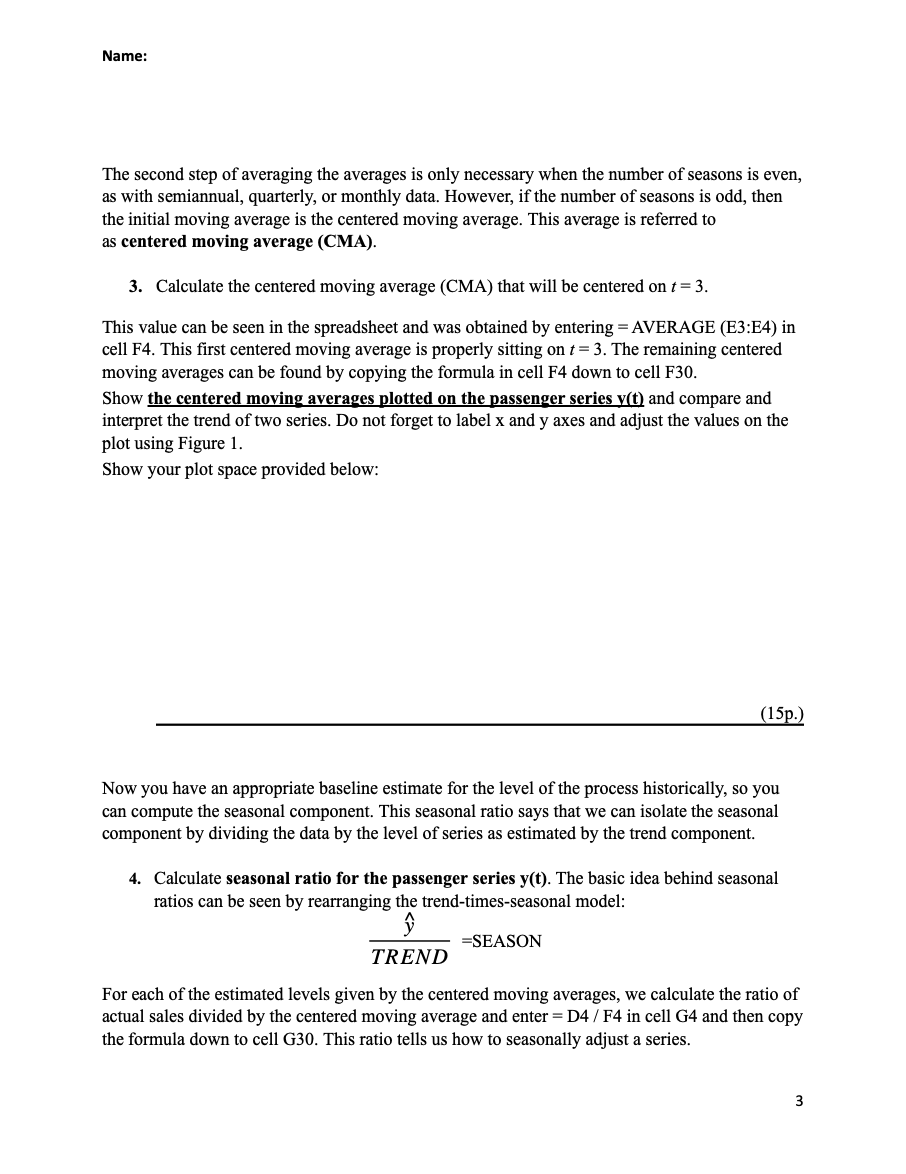
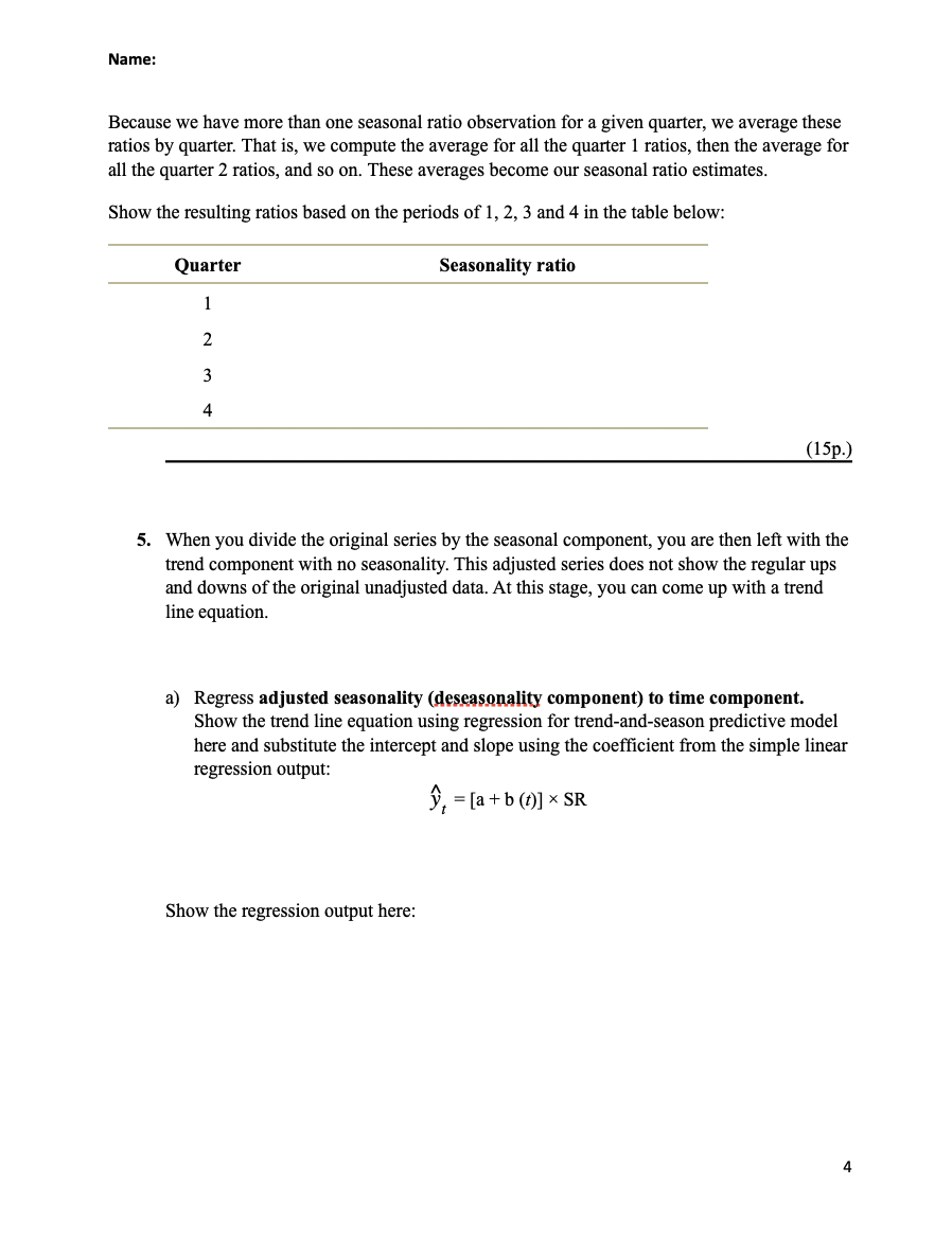
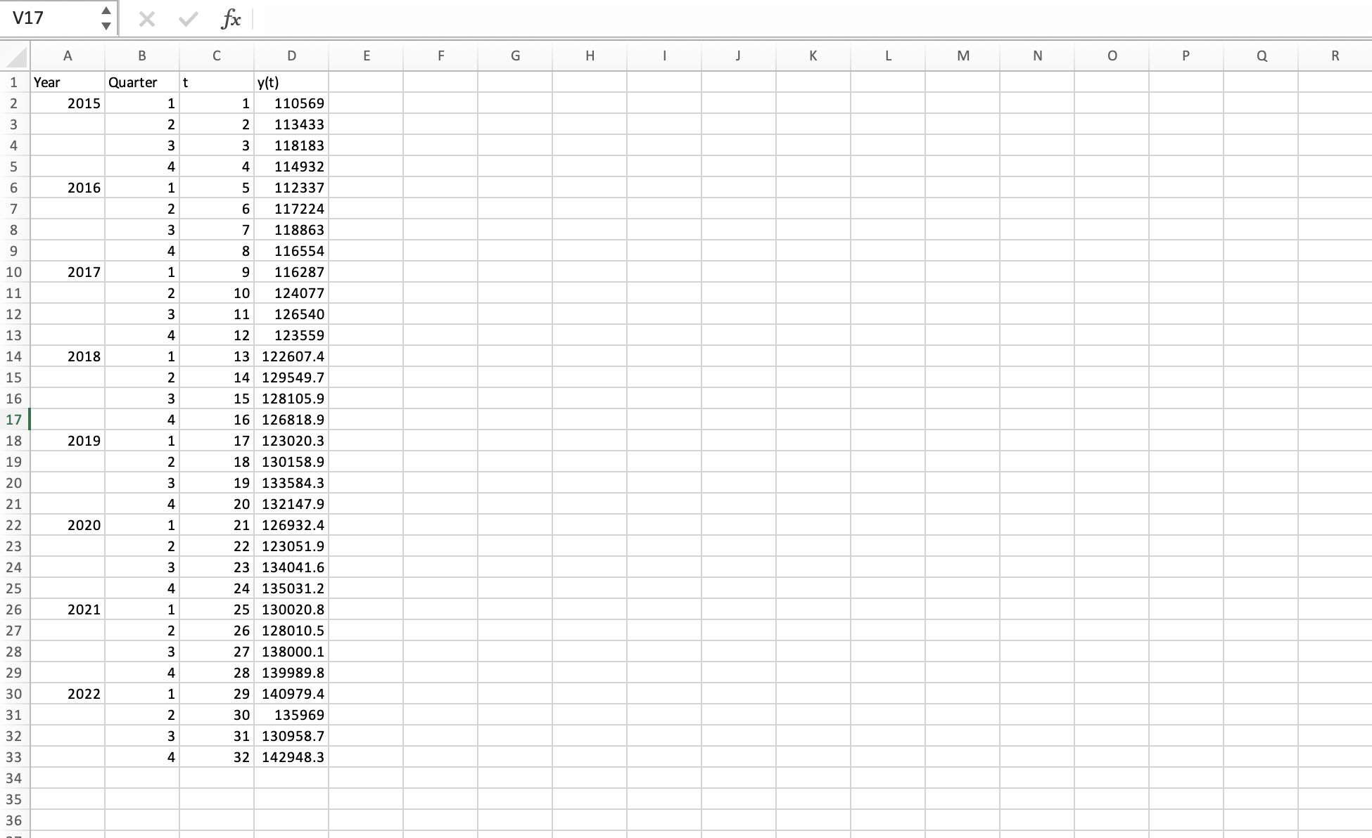
Figure 1. below displays the quarterly number of U.S. passengers (in thousands) using light rail as a mode of transportation. The series begins in the first quarter of 2015 and ends with the last quarter of 2022. We can see a regularity to the series: the first quarter's ridership tends to be lowest; then there is a progressive rise in ridership going into the second and third quarters, followed by a decline in the fourth quarter. Superimposed on the series are the moving-average forecasts based on a span of k=4. Notice that the seasonal pattern in the time series is not present in the moving averages. The moving averages are a smoothed-out version of the original time series, reflecting only the general trend in the series, which is upward. Data Analysis Questions: 1. Calculate the moving averages for each observation in the data based on periods 1,2,3, and 4 . It should be centered on period t=2. Use the function of =AVERAGE (D2:D5) in cell E3 and copy the formula down to cell E31. Show the moving averages plotted on the passenger series y(t). Do not forget to label x and y axes and adjust the values on the plot using Figure1. Show your plot space provided below: (10p.) 2. Even though the moving averages help highlight the long-run trend of a time series, the moving-average model is not designed for making forecasts in the presence of trends. Explain the reason why we should not rely on moving averages for predicting future observations of a trending series. The second step of averaging the averages is only necessary when the number of seasons is even, as with semiannual, quarterly, or monthly data. However, if the number of seasons is odd, then the initial moving average is the centered moving average. This average is referred to as centered moving average (CMA). 3. Calculate the centered moving average (CMA) that will be centered on t=3. This value can be seen in the spreadsheet and was obtained by entering = AVERAGE (E3:E4) in cell F4. This first centered moving average is properly sitting on t=3. The remaining centered moving averages can be found by copying the formula in cell F4 down to cell F30. Show the centered moving averages plotted on the passenger series y(t) and compare and interpret the trend of two series. Do not forget to label x and y axes and adjust the values on the plot using Figure 1. Show your plot space provided below: (15p.) Now you have an appropriate baseline estimate for the level of the process historically, so you can compute the seasonal component. This seasonal ratio says that we can isolate the seasonal component by dividing the data by the level of series as estimated by the trend component. 4. Calculate seasonal ratio for the passenger series y(t). The basic idea behind seasonal ratios can be seen by rearranging the trend-times-seasonal model: TRENDy^=SEASON For each of the estimated levels given by the centered moving averages, we calculate the ratio of actual sales divided by the centered moving average and enter = D4 / F4 in cell G4 and then copy the formula down to cell G30. This ratio tells us how to seasonally adjust a series. Because we have more than one seasonal ratio observation for a given quarter, we average these ratios by quarter. That is, we compute the average for all the quarter 1 ratios, then the average for all the quarter 2 ratios, and so on. These averages become our seasonal ratio estimates. Show the resulting ratios based on the periods of 1,2,3 and 4 in the table below: (15p.) 5. When you divide the original series by the seasonal component, you are then left with the trend component with no seasonality. This adjusted series does not show the regular ups and downs of the original unadjusted data. At this stage, you can come up with a trend line equation. a) Regress adjusted seasonality (deseasonality component) to time component. Show the trend line equation using regression for trend-and-season predictive model here and substitute the intercept and slope using the coefficient from the simple linear regression output: y^t=[a+b(t)]SR Show the regression output here: b) Create a plot using adjusted seasonality (deseasonality component) along with linear trend fit and interpret the graph. Show your plot space provided below and do not forget to label x and y axes and adjust the values on the plot using Figure 1 . (15p.) c) Compute a forecast that the series ended in the last quarter of 2022 with t=32. This means that the next period in the future is the first quarter of 2023 with t=33. y^t=[a+b(t)]SR=? where SR is the seasonality ratio for the appropriate quarter corresponding to the value of t