hello can someone help me with 12 given the data below, parts a-h are marked in red to see easier.

here is the previous work done if needed

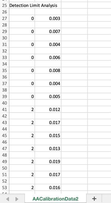
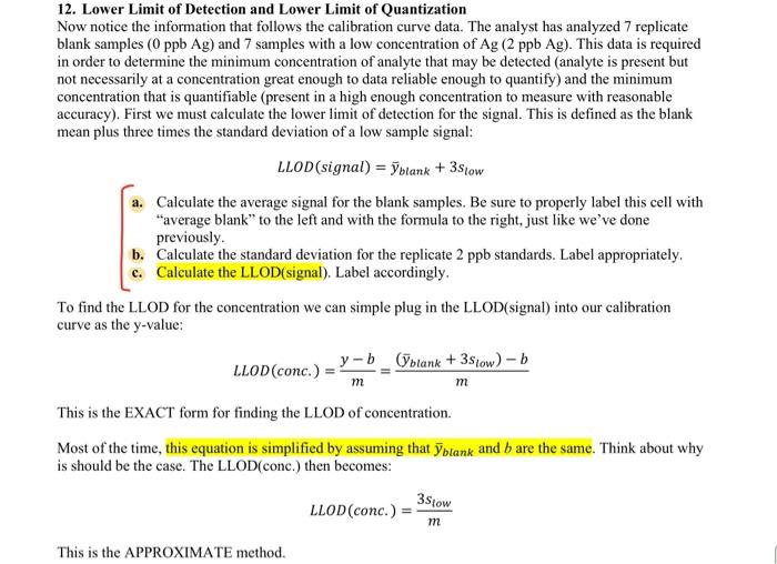
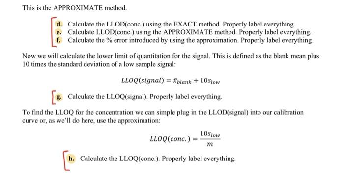
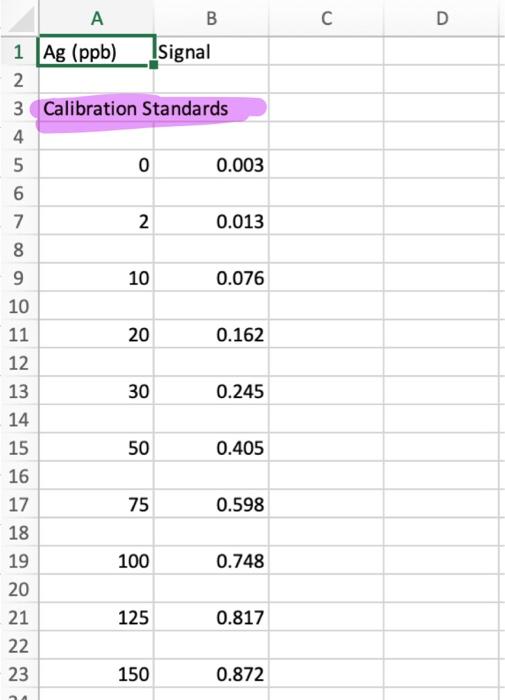
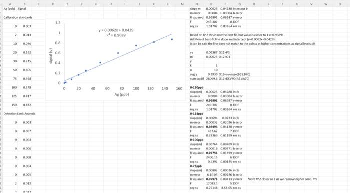
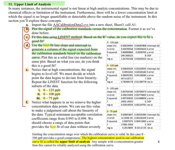
0 25 Detection Limit Analysis 26 27 0 0.003 28 29 0 0.007 30 31 0 0.004 32 33 0 0.006 34 35 0 0.008 36 37 0 0.004 38 39 0 0.005 40 41 2 0.012 42 43 2 0.017 44 45 2 0.015 46 2 0.013 48 49 0.019 50 51 2 0.017 52 53 2 0.016 2 47 2 N N CA AACalibration Data2 + 12. Lower Limit of Detection and Lower Limit of Quantization Now notice the information that follows the calibration curve data. The analyst has analyzed 7 replicate blank samples (0 ppb Ag) and 7 samples with a low concentration of Ag (2 ppb Ag). This data is required in order to determine the minimum concentration of analyte that may be detected (analyte is present but not necessarily at a concentration great enough to data reliable enough to quantify) and the minimum concentration that is quantifiable (present in a high enough concentration to measure with reasonable accuracy). First we must calculate the lower limit of detection for the signal. This is defined as the blank mean plus three times the standard deviation of a low sample signal: LLOD(signal) = Yblank + 3Stow a. Calculate the average signal for the blank samples. Be sure to properly label this cell with "average blank" to the left and with the formula to the right, just like we've done previously. b. Calculate the standard deviation for the replicate 2 ppb standards. Label appropriately. c. Calculate the LLOD(signal). Label accordingly. To find the LLOD for the concentration we can simple plug in the LLOD(signal) into our calibration curve as the y-value: y-b prank + 3Stow) - b LLOD(conc.) m This is the EXACT form for finding the LLOD of concentration. Most of the time, this equation is simplified by assuming that Iblank and b are the same. Think about why is should be the case. The LLOD(conc.) then becomes: 3Slow LLOD(conc.) m This is the APPROXIMATE method. This is the APPROXIMATE method. d. Calculate the LLOD(conc.) using the EXACT method. Properly label everything. e. Calculate LLOD(conc.) using the APPROXIMATE method. Properly label everything. f. Calculate the % error introduced by using the approximation. Properly label everything. Now we will calculate the lower limit of quantitation for the signal. This is defined as the blank mean plus 10 times the standard deviation of a low sample signal: LLOQ(signal) = intank + 10Stow Calculate the LLOQ(signal). Properly label everything. To find the LLOQ for the concentration we can simple plug in the LLOD(signal) into our calibration curve or, as we'll do here, use the approximation: LLOQ(conc.) = m h. Calculate the LLOQ(conc.). Properly label everything. 10stow D A B 1 Ag (ppb) Signal 2. 3 Calibration Standards 4 5 o 0.003 6 7 2 0.013 8 9 10 0.076 10 11 20 0.162 12 13 30 0.245 14 15 50 0.405 16 17 75 0.598 18 19 100 0.748 20 21 125 0.817 22 23 150 0.872 D Atap Spal Caration standards Hope 0.00035 0.04288 tot mer 0.0004 0.01004 squared 0.291 0.06387 verre . 20.301 * DOI 1.0172 0.034 12 1 0 0.003 1 2 0.013 y0.0062x 0,0429 R 0.9689 10 0.096 0.8 Based on this is the best but ve doser to 1968 Addition of best dit line slope and intercepty.001.10.04 can be said the line does not match to the points at light concentrations as signals of w 0.0637 011-23 m 0.0005 012-01 Y & 20 0.162 0.6 signalu) 30 0.245 04 50 0.405 02 75 OS 100 0.74 O 0 20 40 60 100 120 140 160 80 Ag (ppb) 125 11 150 0372 Senimas 1 0 0.003 10 NEY 0.016-061:8700 und 1601.DEVSFA61A/01 0-15b open! 0.0005 0.0128 into mer 0.0004 0.01001 sard 0.96391 0.037 yarro 249.107 8 DO 101702001264 0-125 openi 0.0064 0.023 mero 0.0002 0.00026 ar 0.99401 0011 verre > DO R 0.0119 0-100 000764 000 0.00016 0.00m ben 0.00751 0.01 yir 2400 15 0.51 0.0015 0-75 on 0.0002 0.00036 mer 6.11.05 0.00226 sed 0.99971 0.00033 yr 2 cols were her conch F 170833 0.2941&S 0.007 VES 0 000 0.00 000 100 0.004 0.005 2 0.012 100S Rsquared F reg ss 249.306525 8 DOF merror 11. Upper Limit of Analysis In many instances, the instrumental signal is not linear at high analyte concentrations. This may be due to chemical effects or limitation of the instrument. Furthermore, there will be a lower concentration limit at which the signal is no longer quantifiable or detectable above the random noise of the instrument. In this section you'll explore these concepts. a. Import the file AACalibrationData2.cvs into a new sheet, Sheet3, cell Al. Plot the signal of the calibration standards versus the concentration. Format it as we've done before. Fit this data using LINEST method. Based on the Rvalue, do you expect this to be a good fit? 0-150 ppb d. Use the best-fit line slope and intercept to slope (m) 0.00624594 0.04287808 intercept (b) generate a column of the signal expected from merror 0.00039558 0.03003626b error 0.96890868 0.0638702 y error the calibration standards based on the calibration curve. Plot this as a solid line (no markers) on the 1.01702168 0.03263522 res ss same plot. Based on what you see, do you think this is a good fit? 0-125 ppb e. Notice that at high concentrations, the signal slope (m) 0.00693529 0,02329555 Intercept (b) 0.0003242 0.02026182 berror begins to level off. We must decide at which Rsquared 0.98493392 0.04138284 y error point the data begins to deviate from linearity. 457.619717 7 DOF Repeat the LINEST function for the following reg ss 0.78369178 0.01198778 resss subsets of the data. 0-100 ppb i. 0-125 ppb slope (m) 0.00764196 0.00709473 intercept (b) ii. 0-100 ppb merror 0.00015599 0.00770692 b error iii. 0-75 ppb Rsquared 0.99750639 0.01498836 y error f. Notice what happens to as we remove the higher 2400.14923 6 DOF 0.53919559 0.00134791 resss concentration data points. We can use this value to make a judgement call about the linearity of 0.75 ppb the data. Typical minimum acceptable correlation slope (m) 0.00801847 0.00036384 intercept (b) coefficients range from 0.995 to 0.999. We merror 6.1349E-05 0.00226349 b error Rsquared 0.9997074 0.00413065 y error should choose a range of data points that 17083.3458 provides the best fit of our data without severely regs 0.2914804 8.5311E-05 resss limiting the concentration range over which the calibration curve is valid. In this case 0 - 100 ppb provides a good compromise. The highest concentration used in our calibration curve fit is called the upper limit of analysis. Any sample with a concentration greater than this cannot be reliably analyzed using the calibration curve. reg ss 5 DOF 8