Hello,please help me solve these steps by explaining how to perform

these steps in excel in detail. Please explain every step

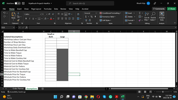
thoroughly also explain each formula and how to use it$.$Click on the Assumptions Tab and enter the isolated assumption

values using the information from the problem description above.

Every cell should have a value.

$5.$ The Hours per Day Available for the Small Shop is calculated in

cell C$5$ as the Number of Shop Workers times the Workshop Hours per

Day $$ both assumptions found on the Assumption tab. Using the

mouse, construct the formula so it looks like:

$=$Assumptions!C$3*$Assumptions$!$C$4$

Modify the formula so that the cell references are partially

absolute $$ that is the row number is anchored $($has a $ sign in

front of it$)$ but the column letter is not.

$6.$ Calculate in C$6$ the Daily Labour Cost for the Small Shop as the

Hours per Day Available times the Workshop Labour Cost per Hour $($an

assumption$).$ Again, this should use only a partial absolute

reference to the assumption value $$ anchoring just the row

number.

$7.$ In cell C$13,$ we need to calculate the total number of hours it

will take to produce the item indicated in cells C$8$:C$11.$ Even

though cells C$10$ and C$11$ will only ever be $0,$ we want to be sure

the formula covers all options. Create a formula that adds together

the products of the Number of Items being made times the Time to

Make assumption associated with that item.

The formula should look something like this $($not the complete

formula$)$:

$=$ C$8*$Assumptions$!$$C$$6+$ C$9*$Assumptions$!$$C$$7+...$

$8.$ The Total Wholesale Value in cell C$16$ and the Total Material

Cost in cell C$19$ are calculated in a similar manner. The Wholesale

Value is the result of multiplying the number

of each item by its respective Wholesale Price found in the

assumptions $$ and then adding all those products together.

Likewise, the Total Material Cost multiplies the number of each

item being produced by its associated Material Cost value in the

assumptions and adds those together. Enter formulas for both cells

and make sure all references to assumptions are fully anchored so

they are absolute references.

$9.$ Next calculate the Total Shop Days in cell C$14$ for the Small

Workshop as the Production Man Hours divided by the Hours per Day

Available for the shop.

$10.$ The Total Labour Cost in cell C$18$ is found by multiplying the

Production Man Hours by Workshop Labour Cost per Hour. Finally, the

Total Overhead Cost is found by multiplying the Total Shop Days by

the associated Workshop Daily Overhead Cost. All references to

assumptions must be partially anchored references $($only on the

row$).$

$11.$ Now sum up the Total Costs in C$21$ using a sum function $$

summing up cells C$18,$ C$19$ & C$20.$ Next calculate the Gross

Profit as Total Wholesale Value $($C$16)$ minus Total Costs

$($C$21).$

Figure Q$1-1$

$12.$ Copy cells C$5$:C$6$ into D$5$:D$6.$ Likewise, copy C$13$:C$23$ into

D$13$:D$23.$

$13.$ The final step in creating this Order Planner worksheet is to

create all the Total formulas. In cell F$8,$ enter $=$C$8+$D$8.$ Do the

same in cells F$9$:F$11,$ F$13$:F$14,$ F$16,$ F$18$:F$21,$ and F$23.$ If you

populate cells C$9,$ C$11,$ D$8$:D$11$ with ones, the final version of the

worksheet should look like Figure Q$1-1.$ You may need to copy the

formatting from cells D$13$:D$23$ over to F$13$:F$23.$

$14.$ Save your work at this.

$15.$ Next, we want to use the tool to determine several order plans.

Below is a table detailing three order plans. The instructions will

help you work through the first one $$ and then you will complete

the other two $$ following which, you will generate a Scenario

Manager Summary Report. Order $1$ Order $2$ Order $3$ Baseball Caps $50$

$300125$

Toques

$20$

$75$

$100$ Fedoras $125025$

Cowboy Hats

$15$

$20$

$25$ Max Days to Complete $2\mathrm{.}57\mathrm{.}255\mathrm{.}5$

$16.$ Enter the Order $1($or the next order$)$ details into cells

C$28$:C$32.$

$17.$ Enter zeros into cells C$8,$ C$9,$ and D$8$:D$11.$

$18.$ Now we want to open the Solver tool. Select Solver from the

Analyze Group on the Data Ribbon. Our objective for this Order

Planner tool will be to have minimum total costs while determining

the values for cells C$8,$ C$9,$ D$8,$ D$9,$ D$10$ and D$11.$ In the solver

tool,

a$.$ select the Set Objective box, then click on cell F$21$ to enter

this as the objective cell.

b$.$ Next select Min to indicate that we want this cell to be as

small as possible.

c$.$ Select the By Changing Variable Cells box $$ and then while

holding down the Ctrl$-$Key, select cells C$8,$ C$9,$ D$8,$ D$9,$ D$10$ and D$11$

$($the variable cells$).$

d$.$ Click the Add button to start adding constraints. You will need

the following:

i$.6$ constraints requiring the variable cells to be integers

$($int$)$

ii$.6$ constraints requiring the variable cells to be greater than

or equal to zero.

iii. $4$ constraints requiring each of the totals in cells F$8$:F$11$ to

be equal to the order requirements in cells C$28$:C$31$ respectively.

The cell F$8$ must equal cell C$28,$ cell F$9$ must equal cell C$29,$

etc...

iv$.2$ constraints restricting the Total Shop Days values in C$14$ and

D$14$ to be less than or equal to the Max Days to Complete value in

C$32.$

$19.$ Using the Simplex LP method, solve for a solution to this

problem. If a solution is found, first save the solution using the

Save Scenario button. Use Order$1$ as the Scenario Name. Then select

Keep the Solution and click on Activity $($or Answer$)$ to generate the

Activity $($or Answer$)$ report. Finally, select OK$.$

$20.$ Open the Scenario Manager $($under the What$-$If$-$Tools list$),$

select Order $1$ and then click Edit. In the Changing Variables

field, add the additional cells of C$28$:C$32.$ Click OK and then

verify that these cells were added to the bottom of the Scenario

Values dialog box $($at the bottom$).$ Once satisfied they were added,

click OK once more.

$21.$ Change the values in cells C$28$:C$32$ for the next order and

repeat steps $16,17,18,19$ and $20$ until all three orders are

done

$22.$ After the three orders are complete, name the following

cells:

F$13$ to Total$\_$Man$\_$Hours,

C$14$ to Small$\_$Shop$\_$Days,

D$14$ to Large$\_$Shop$\_$Days,

F$16$ to Revenue,

F$21$ to Costs, and

F$23$ to Gross$\_$Profit.

$23.$ Finally, we want to generate a Scenario Manager Summary report.

Select the Scenario Manager tool, select the Summary button, and

then select cells F$13,$ C$14,$ D$14,$ F$16,$ F$21,$ and F$23$ as the result

cells to include in the report. Select Scenario Summary and the

click OK$.$

$24.$ You should have the following tabs in your final workbook:

$25.$ Save the changes to the workbook and submit the results to the

course website.