help me in this problems
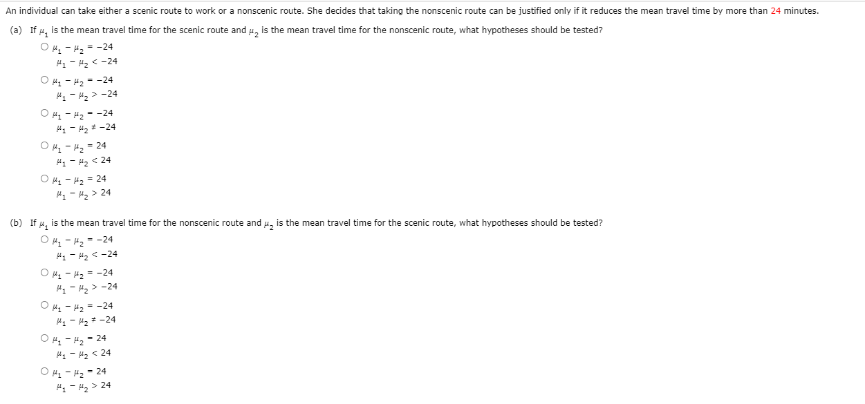
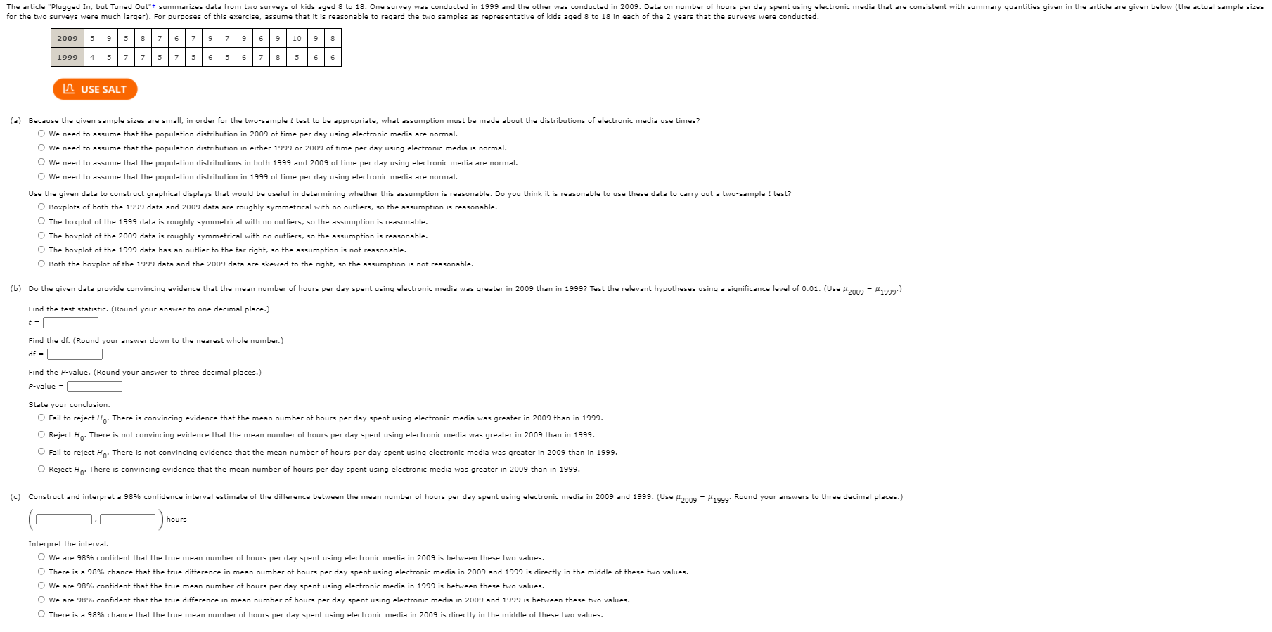
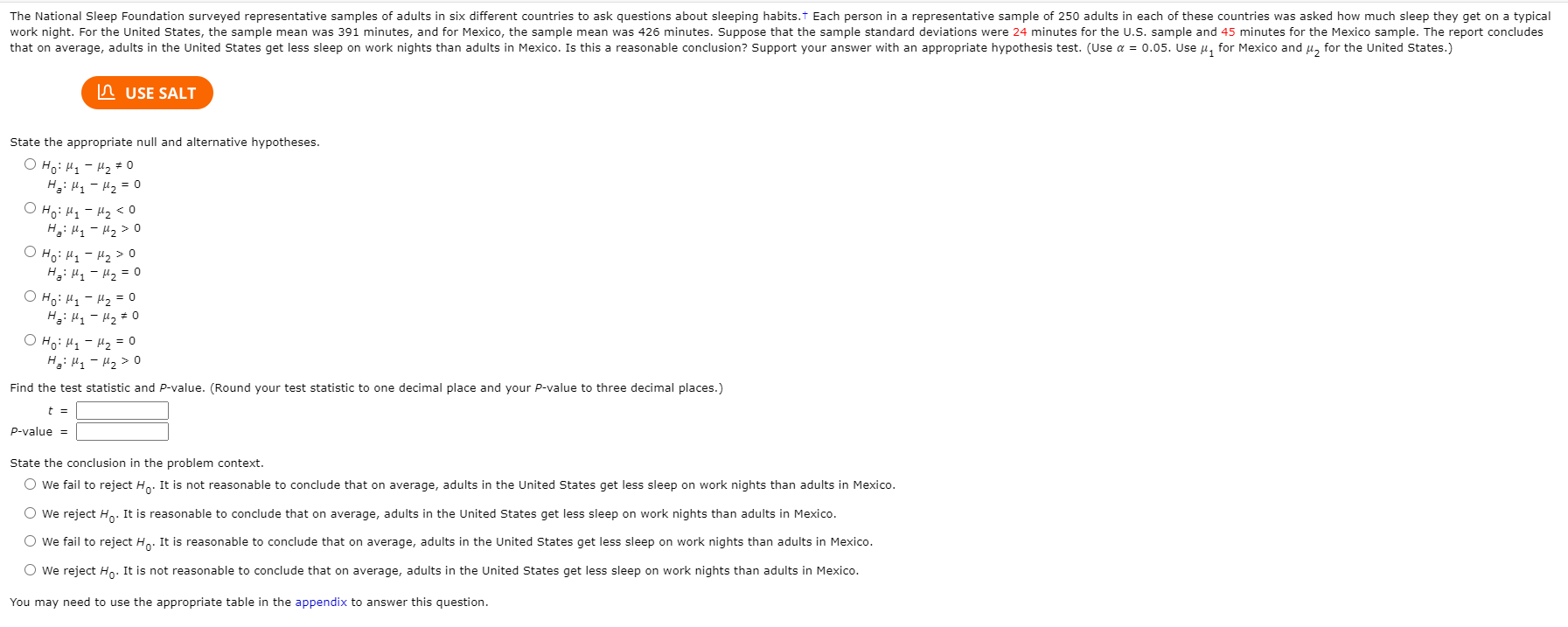
Consider two populations for which u, = 36, , = 3, u, = 23, and , = 2. Suppose that two independent random samples of sizes n, = 43 and n, = 55 are selected. Describe the approximate sampling distribution of x, - X, (center, variability, and shape). What is the shape of the distribution? O The distribution would be non-normal. O The distribution is approximately normal. O The shape cannot be determined. What is the mean of the distribution? What is the standard deviation of the distribution? (Round your answer to three decimal places.)An individual can take either a scenic route to work or a nonscenic route. She decides that taking the nonscenic route can be justified only if it reduces the mean travel time by more than 24 minutes. (a) If u, is the mean travel time for the scenic route and u, is the mean travel time for the nonscenic route, what hypotheses should be tested? OH1 - H2 = -24 Hy - H2 -24 OH1 - H2 = -24 H1 - H2 # -24 OH, - 4, = 24 Hy - Hz 24 (b) If u, is the mean travel time for the nonscenic route and u, is the mean travel time for the scenic route, what hypotheses should be tested? OH, - H2 = -24 Hy - H2 -24 OH1 - 42 = -24 H1 - H2 # -24 OH, - H, = 24 H1 - H2 24The article "Plugged In, but Tuned Out"t summarizes data from two surveys of kids aged 8 to 18. One survey was conducted in 1999 and the other was conducted in 2009. Data on number of hours per day spent using electronic media that are consistent with summary quantities given in the article are given below (the actual sample sizes for the two surveys were much larger). For purposes of this exercise, assume that it is reasonable to regard the two samples as representative of kids aged 8 to 18 in each of the 2 years that the surveys were conducted. 2009 5 9 5 8 7 6 7 9 7 9 6 9 10 9 8 1999 4 5 7 7 5 7 5 6 5 6 7 8 5 6 6 LA USE SALT (a) Because the given sample sizes are small, in order for the two-sample & test to be appropriate, what assumption must be made about the distributions of electronic media use times? O We need to assume that the population distribution in 2009 of time per day using electronic media are normal. O We need to assume that the population distribution in either 1999 or 2009 of time per day using electronic media is normal. We need to assume that the population distributions in both 1999 and 2009 of time per day using electronic media are normal. O We need to assume that the population distribution in 1999 of time per day using electronic media are normal. Use the given data to construct graphical displays that would be useful in determining whether this assumption is reasonable. Do you think it is reasonable to use these data to carry out a two-sample t test? O Boxplots of both the 1999 data and 2009 data are roughly symmetrical with no outliers, so the assumption is reasonable. O The boxplot of the 1999 data is roughly symmetrical with no outliers, so the assumption is reasonable. O The boxplot of the 2009 data is roughly symmetrical with no outliers, so assumption is reasonable. O The boxplot of the 1999 data has an outlier to the far right, so the assumption is reasonable. O Both the boxplot of the 1999 data and the 2009 data are skewed to the right, so the assumption is not reasonable. (b) Do the given data provide convincing evidence that the mean number of hours per day spent using electronic media was greater in 2009 than in 1999? Test the relevant hypotheses using a significance level of 0.01. (Use /2009 - #1999.) Find the test statistic. (Round your answer to one decimal place.) Find the df. (Round your answer down to the nearest whole number.) If = Find the P-value. (Round your answer to three decimal places.) P-value =| State your conclusion. O Fail to reject Ho. There is convincing evidence that the mean number of hours per day spent using electronic media was greater in 2009 than in 1999. O Reject Ho. There is not convincing evidence that the mean number of hours per day spent using electronic media was greater in 2009 than in 1999. O Fail to reject Ho. There is not convincing evidence that the mean number of hours per day spent using electronic media was greater in 2009 than in 1999. O Reject Ho. There is convincing evidence that the mean number of hours per day spent using el media was greater in 2009 than in 1999. (c) Construct and interpret a 98% confidence interval estimate of the difference between the mean number of hours per day spent using electronic media in 2009 and 1999. (Use #2009 - #jggg. Round your answers to three decimal places.) hours Interpret the interval. We are 98% confident that the true mean number of hours per day spent using electronic media in 2009 is between these two values. O There is a 98% chance that the true difference in mean number of hours per day spent using electronic media in 2009 and 1999 is directly in the middle of these two values. O We are 98% confident that the true mean number of hours per day spent using electronic media in 1999 is between these two values. O We are 98% confident that the true difference in mean number of hours per day spent using electronic media in 2009 and 1999 is between these two values. There is a 98% chance that the true mean number of hours per day spent using electronic media in 2009 is directly in the middle of these two values.The National Sleep Foundation surveyed representative samples of adults in six different countries to ask questions about sleeping habits. Each person in a representative sample of 250 adults in each of these countries was asked how much sleep they get on a typical work night. For the United States, the sample mean was 391 minutes, and for Mexico, the sample mean was 426 minutes. Suppose that the sample standard deviations were 24 minutes for the U.S. sample and 45 minutes for the Mexico sample. The report concludes that on average, adults in the United States get less sleep on work nights than adults in Mexico. Is this a reasonable conclusion? Support your answer with an appropriate hypothesis test. (Use a = 0.05. Use #, for Mexico and #2 for the United States.) LA USE SALT State the appropriate null and alternative hypotheses. O Ho: H1 - H2 = 0 Ha: H1 - H2 = 0 O HO: H 1 - H2 0 OH: H - H2 > 0 Ha: H 1 - H2 = 0 OH: H1 - H2 = 0 Ha: H 1 - H2 = 0 OHO: H1 - H2 = 0 Ha: H 1 - H2 > 0 Find the test statistic and P-value. (Round your test statistic to one decimal place and your P-value to three decimal places.) P-value = State the conclusion in the problem context. O We fail to reject Ho. It is not reasonable to conclude that on average, adults in the United States get less sleep on work nights than adults in Mexico. O We reject H . It is reasonable to conclude that on average, adults in the United States get less sleep on work nights than adults in Mexico. We fail to reject Ho. It is reasonable to conclude that on average, adults in the United States get less sleep on work nights than adults in Mexico. We reject Ho. It is not reasonable to conclude that on average, adults in the United States get less sleep on work nights than adults in Mexico. You may need to use the appropriate table in the appendix to answer this question.The paper "If It's Hard to Read, It's Hard to Do"t described an interesting study of how people perceive the effort required to do certain tasks. Each of 20 students was randomly assigned to one of two groups. One group was given instructions for an exercise routine that were printed in an easy-to-read font (Arial). The other group received the same set of instructions, but printed in a font that is considered difficult to read (Bruck). After reading the instructions, subjects estimated the time (in minutes) they thought it would take to complete the exercise routine. Summary statistics are given below. Easy Font Difficult Font 10 10 8.23 15.10 5.61 9.28 The authors of the paper used these data to carry out a two-sample t test, and concluded that at the 0.10 significance level, there was convincing evidence that the mean estimated time to complete the exercise routine was less when the instructions were printed in an easy-to-read font than when printed in a difficult-to-read font. Discuss the appropriateness of using a two-sample t test in this situation. The treatment groups were small, so in order to use the two-sample t test it is necessary to assume that the population distributions of estimated times for each group are normal. However, in both samples zero is about 1.5 standard deviations below the mean. If we assume that the populations have means and standard deviations equal to the sample means and standard deviations, this would imply that almost all of people in each population have positive estimated times. Since we can only have positive times, this supports the assumption that the populations are approximately normally distributed and the two-sample t test is appropriate. The treatment groups were small, so in order to use the two-sample t test it is necessary to assume that the population distributions of estimated times for each group are normal. However, in both samples zero is about 3 standard deviations below the mean. If we assume that the populations have means and standard deviations equal to the sample means and standard deviations, this would imply that a significant proportion of people in each population have negative estimated times. Since this is impossible, the populations are unlikely to be approximately normally distributed and the two-sample t test is not appropriate. The treatment groups were small, so in order to use the two-sample t test it is necessary to assume that the population distributions of estimated times for each group are normal. However, in both samples zero is about 3 standard deviations below the mean. If we assume that the populations have means and standard deviations equal to the sample means and standard deviations, this would imply that almost all of people in each population have positive estimated times. Since we can only have positive times, this supports the assumption that the populations are approximately normally distributed and the two-sample t test is appropriate. The treatment groups were small, so in order to use the two-sample t test it is necessary to assume that the population distributions of estimated times for each group are normal. However, in both samples zero is about 1.5 standard deviations below the mean. If we assume that the populations have means and standard deviations equal to the sample means and standard deviations, this would imply that a significant proportion of people in each population have negative estimated times. Since this is impossible, the populations are unlikely to be approximately normally distributed and the two-sample t test is not appropriate


