$$help me solve this pls.

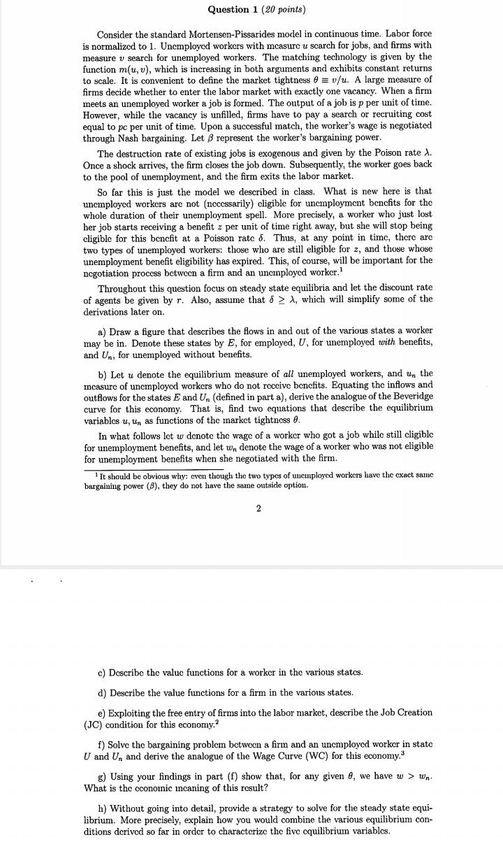
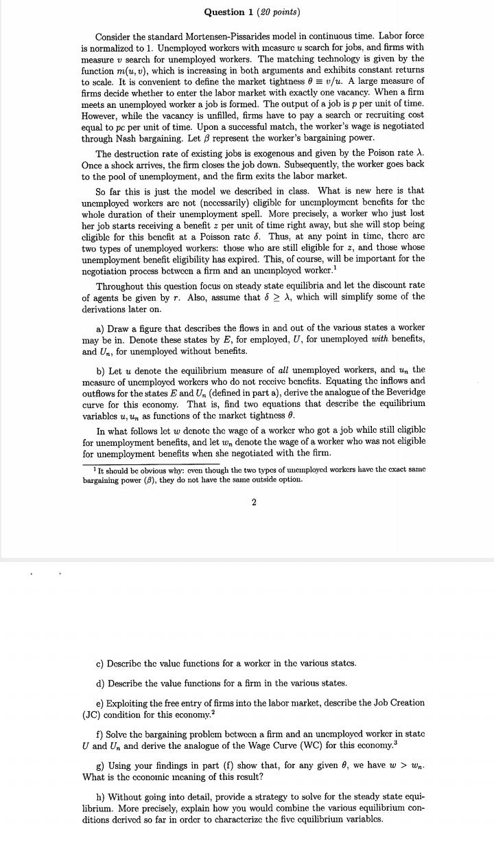
Question 1 (20 points) Consider the standard Mortensen-Pissarides model in continuous time. Labor force is normalized to 1. Unemployed workers with measure u search for jobs, and firms with measure v search for unemployed workers. The matching technology is given by the function m(u, v), which is increasing in both arguments and exhibits constant returns to scale. It is convenient to define the market tightness 0 = v/u. A large measure of firms decide whether to enter the labor market with exactly one vacancy. When a firm meets an unemployed worker a job is formed. The output of a job is p per unit of time. However, while the vacancy is unfilled, firms have to pay a search or recruiting cost equal to pc per unit of time. Upon a successful match, the worker's wage is negotiated through Nash bargaining. Let / represent the worker's bargaining power. The destruction rate of existing jobs is exogenous and given by the Poison rate A. Once a shock arrives, the firm closes the job down. Subsequently, the worker goes back to the pool of unemployment, and the firm exits the labor market. So far this is just the model we described in class. What is new here is that unemployed workers are not (necessarily) eligible for unemployment benefits for the whole duration of their unemployment spell. More precisely, a worker who just lost her job starts receiving a benefit z per unit of time right away, but she will stop being eligible for this benefit at a Poisson rate o. Thus, at any point in time, there are two types of unemployed workers: those who are still eligible for z, and those whose unemployment benefit eligibility has expired. This, of course, will be important for the negotiation process between a firm and an unemployed worker. Throughout this question focus on steady state equilibria and let the discount rate of agents be given by r. Also, assume that o 2 A, which will simplify some of the derivations later on. a) Draw a figure that describes the flows in and out of the various states a worker may be in. Denote these states by E, for employed, U, for unemployed with benefits, and Un, for unemployed without benefits. b) Let u denote the equilibrium measure of all unemployed workers, and un the measure of unemployed workers who do not receive benefits. Equating the inflows and outflows for the states E and Un (defined in part a), derive the analogue of the Beveridge curve for this economy. That is, find two equations that describe the equilibrium variables u, un as functions of the market tightness e. In what follows lot w denote the wage of a worker who got a job while still eligible for unemployment benefits, and let w, denote the wage of a worker who was not eligible for unemployment benefits when she negotiated with the firm. 1 It should be obvious why: even though the two types of unemployed workers have the exact same bargaining power (8), they do not have the same outside option. 2 c) Describe the value functions for a worker in the various states. d) Describe the value functions for a firm in the various states. e) Exploiting the free entry of firms into the labor market, describe the Job Creation (JC) condition for this economy.' f) Solve the bargaining problem between a firm and an unemployed worker in state U and Un and derive the analogue of the Wage Curve (WC) for this economy. g) Using your findings in part (f) show that, for any given 0, we have w > wn. What is the economic incaning of this result? h) Without going into detail, provide a strategy to solve for the steady state equi- librium. More precisely, explain how you would combine the various equilibrium con- ditions derived so far in order to characterize the five equilibrium variables.Question 1 (20 points) Consider the standard Mortensen-Pissarides model in continuous time. Labor force is normalized to 1. Unemployed workers with measure u search for jobs, and firms with measure u search for unemployed workers. The matching technology is given by the function m(u, v), which is increasing in both arguments and exhibits constant returns to scale. It is convenient to define the market tightness 0 = v/u. A large measure of firms decide whether to enter the labor market with exactly one vacancy. When a firm meets an unemployed worker a job is formed. The output of a job is p per unit of time. However, while the vacancy is unfilled, firms have to pay a search or recruiting cost equal to pc per unit of time. Upon a successful match, the worker's wage is negotiated through Nash bargaining. Let / represent the worker's bargaining power. The destruction rate of existing jobs is exogenous and given by the Poison rate X. Once a shock arrives, the firm closes the job down. Subsequently, the worker goes back to the pool of unemployment, and the firm exits the labor market. So far this is just the model we described in class. What is new here is that unemployed workers are not (necessarily) eligible for unemployment benefits for the whole duration of their unemployment spell. More precisely, a worker who just lost her job starts receiving a benefit z per unit of time right away, but she will stop being eligible for this benefit at a Poisson rate o. Thus, at any point in time, there are two types of unemployed workers: those who are still eligible for z, and those whose unemployment benefit eligibility has expired. This, of course, will be important for the negotiation process between a firm and an unemployed worker.' Throughout this question focus on steady state equilibria and let the discount rate of agents be given by r. Also, assume that o 2 1, which will simplify some of the derivations later on. a) Draw a figure that describes the flows in and out of the various states a worker may be in. Denote these states by E, for employed, U, for unemployed with benefits, and Un, for unemployed without benefits. b) Let u denote the equilibrium measure of all unemployed workers, and un the measure of unemployed workers who do not receive benefits. Equating the inflows and outflows for the states E and Un (defined in part a), derive the analogue of the Beveridge curve for this economy. That is, find two equations that describe the equilibrium variables u, un as functions of the market tightness 0. In what follows let w denote the wage of a worker who got a job while still eligible for unemployment benefits, and let w, denote the wage of a worker who was not eligible for unemployment benefits when she negotiated with the firm. ' It should be obvious why: even though the two types of uncinployed workers have the exact same bargaining power (8), they do not have the same outside option. 2 c) Describe the value functions for a worker in the various states. d) Describe the value functions for a firm in the various states. e) Exploiting the free entry of firms into the labor market, describe the Job Creation (JC) condition for this economy.' f) Solve the bargaining problem between a firm and an unemployed worker in state U and Un and derive the analogue of the Wage Curve (WC) for this economy. g) Using your findings in part (f) show that, for any given 0, we have w > w.. What is the economic incaning of this result? h) Without going into detail, provide a strategy to solve for the steady state equi- librium. More precisely, explain how you would combine the various equilibrium con- ditions derived so far in order to characterize the five equilibrium variables.Question 2 (20 points) This question studies the co-existence of money and credit. Time is discrete with an infinite horizon. Each period consists of two subperiods. In the day, trade is bilateral and partially anonymous as in Kiyotaki and Wright (1991) (call this the KW market). At night trade takes place in a Walrasian or centralized market (call this the CM). There are two types of agents, buyers and sellers, and the measure of both is normalized to 1. The per period utility for buyers is u(q) + U(X) - H, and for sellers it is -q + U(X) - H, where q is the quantity of the day good produced by the seller and consumed by the buyer, X is consumption of the night good (the numeraire), and H is hours worked in the CM. In the CM, all agents can turn one unit of labor into a unit of good. The functions u, U satisfy the usual assumptions; I will only spell out the most crucial ones: There exists X* E (0, co) such that U'(X*) = 1, and we define the first-best quantity traded in the KW market as q' = (q : u'(q') = 1}. Here we will assume that there are two types of sellers. Type-1 sellers, with measure 1 - o, never accept unsecured credit. Hence, in any meeting with this type of seller, the buyer must pay on the spot (quid pro quo) with money. In contrast, type-2 sellers, with measure o, accept money but they also accept unsecured credit, in the form of a promise by the buyer to repay the seller in the forthcoming CM with numeraire good. However, there is a credit limit: the buyer can credibly promise to repay only an amount up to C 8 - 1. New money is introduced, or withdrawn if a 0. Is this intuition (always) correct in this model and why?10. One-sided search with tenure Time: Discrete, infinite horizon. Demography: Single worker who lives for ever. Preferences: The worker is risk-neutral (i.e. u(x) = r). He discounts the future at the rate Endowments: When unemployed the worker receives income b per period. Also with prob- ability a he gets an offer of employment at a wage w ~- F(.) on [0, w] where u > b. When employed the worker gets laid off (looses his job) with probability X. Also while em- ployed there is a probability y that the worker gets "tenure". When the worker has tenure he is no longer subject to layoff - he keeps his job for ever. (Getting tenure and getting laid off are mutually exclusive events and * + y