Help Please!! The last 2 images I need to fill in. I tried the first part, but may be wrong.

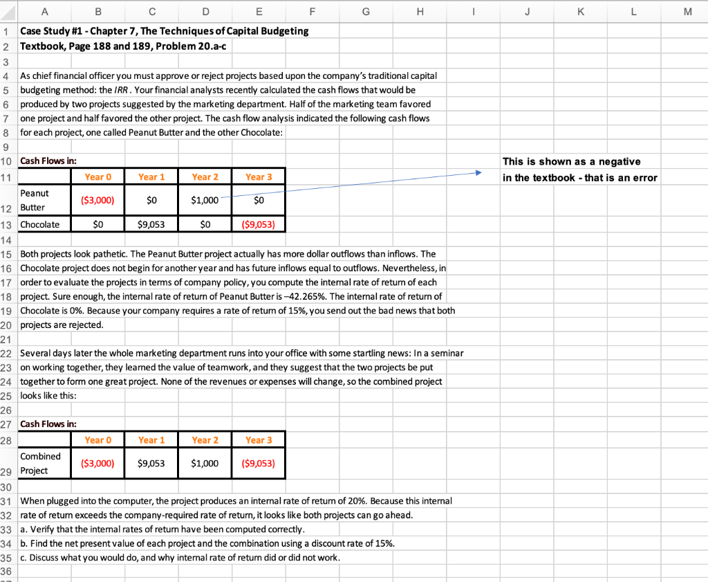
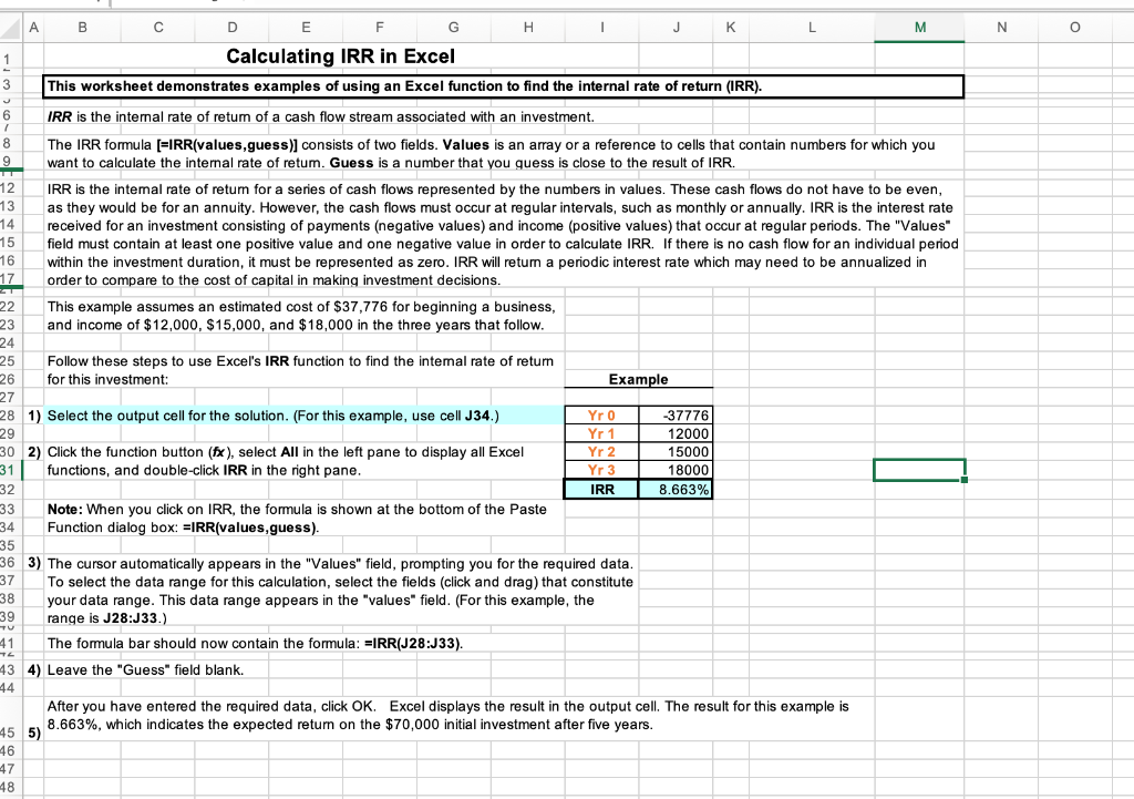
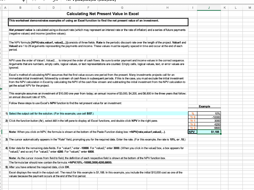
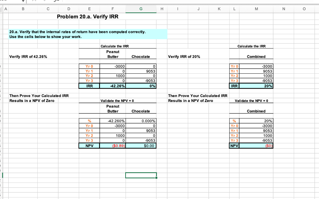
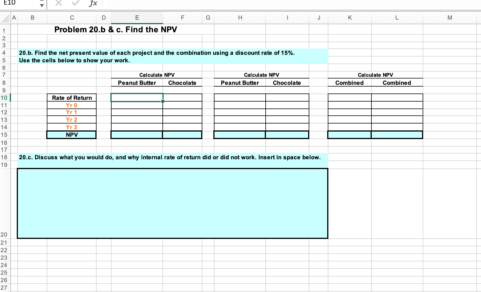
A B 1 Case Study #1 - Chapter 7, The Techniques of Capital Budgeting 2 Textbook, Page 188 and 189, Problem 20.a-c 3 4 As chief financial officer you must approve or reject projects based upon the company's traditional capital budgeting method: the IRR. Your financial analysts recently calculated the cash flows that would be 5 6 produced by two projects suggested by the marketing department. Half of the marketing team favored one project and half favored the other project. The cash flow analysis indicated the following cash flows for each project, one called Peanut Butter and the other Chocolate: 7 8 9 10 Cash Flows in: 11 Peanut 12 Butter Year 0 ($3,000) $0 Year 0 Year 1 $0 ($3,000) $9,053 D Year 1 $9,053 Year 2 $1,000 E 13 Chocolate 14 15 Both projects look pathetic. The Peanut Butter project actually has more dollar outflows than inflows. The 16 Chocolate project does not begin for another year and has future inflows equal to outflows. Nevertheless, in 17 order to evaluate the projects in terms of company policy, you compute the internal rate of return of each 18 project. Sure enough, the internal rate of return of Peanut Butter is -42.265%. The internal rate of return of 19 Chocolate is 0%. Because your company requires a rate of return of 15%, you send out the bad news that both 20 projects are rejected. 21 22 Several days later the whole marketing department runs into your office with some startling news: In a seminar 23 on working together, they learned the value of teamwork, and they suggest that the two projects be put 24 together to form one great project. None of the revenues or expenses will change, so the combined project 25 looks like this: 26 27 Cash Flows in: 28 $0 Year 2 $1,000 Year 3 $0 ($9,053) F Year 3 G H ($9,053) Combined 29 Project 30 31 When plugged into the computer, the project produces an internal rate of return of 20%. Because this internal 32 rate of return exceeds the company-required rate of return, it looks like both projects can go ahead. 33 a. Verify that the internal rates of return have been computed correctly. 34 b. Find the net present value of each project and the combination using a discount rate of 15%. 35 c. Discuss what you would do, and why internal rate of return did or did not work. 36 I J K L This is shown as a negative in the textbook - that is an error M 1 3 J 6 T 8 9 12 13 14 15 16 17 22 23 24 25 26 27 A 41 72 43 44 45 46 B 47 48 F Calculating IRR in Excel This worksheet demonstrates examples of using an Excel function to find the internal rate of return (IRR). IRR is the internal rate of retum of a cash flow stream associated with an investment. The IRR formula [=IRR(values,guess)] consists of two fields. Values is an array or a reference to cells that contain numbers for which you want to calculate the internal rate of retum. Guess is a number that you guess is close to the result of IRR. D 5) E G 28 1) Select the output cell for the solution. (For this example, use cell J34.) 29 H 30 2) Click the function button (fx), select All in the left pane to display all Excel 31 functions, and double-click IRR in the right pane. 32 This example assumes an estimated cost of $37,776 for beginning a business, and income of $12,000, $15,000, and $18,000 in the three years that follow. Follow these steps to use Excel's IRR function to find the internal rate of return for this investment: I IRR is the intemal rate of retum for a series of cash flows represented by the numbers in values. These cash flows do not have to be even, as they would be for an annuity. However, the cash flows must occur at regular intervals, such as monthly or annually. IRR is the interest rate received for an investment consisting of payments (negative values) and income (positive values) that occur at regular periods. The "Values" field must contain at least one positive value and one negative value in order to calculate IRR. If there is no cash flow for an individual period within the investment duration, it must be represented as zero. IRR will return a periodic interest rate which may need to be annualized in order to compare to the cost of capital in making investment decisions. 33 34 35 36 3) The cursor automatically appears in the "Values" field, prompting you for the required data. To select the data range for this calculation, select the fields (click and drag) that constitute 37 38 your data range. This data range appears in the "values" field. (For this example, the range is J28:J33.) 39 The formula bar should now contain the formula: =IRR(J28:J33). 4) Leave the "Guess" field blank. Note: When you click on IRR, the formula is shown at the bottom of the Paste Function dialog box: IRR(values,guess). Example Yr 0 Yr 1 Yr 2 Yr 3 IRR J After you have entered the required data, click OK. 8.663%, which indicates the expected return on the $70,000 initial investment after five years. K -37776 12000 15000 18000 8.663% L M Excel displays the result in the output cell. The result for this example is N O D ? S 3 } 1 1 - 5 B 2 5 NPV uses the order of Value1, Value2,... to interpret the order of cash flows. Be sure to enter payment and income values in the correct sequence. 6 Arguments that are numbers, empty cells, logical values, or text representations are counted. Empty cells, logical values, text, or error values are ignored. - 5 - 6 2 B A 5 F G Calculating Net Present Value in Excel This worksheet demonstrates examples of using an Excel function to find the net present value of an investment. B C D E Net present value is calculated using a discount rate (which may represent an interest rate or the rate of inflation) and a series of future payments (negative values) and income (positive values). H The NPV formula [NPV(rate,value1, value2,...)] consists of three fields. Rate is the periodic discount rate over the length of the project. Value1 and Value2 are 1 to 29 arguments representing the payments and income. These values must be equally spaced in time and occur at the end of each period. Excel's method of calculating NPV assumes that the first value occurs one period from the present. Many investments projects call for an immediate initial investment, followed by a stream of cash flows in subsequent periods. If this is the case, you must exclude the initial investment from the NPV calculation in Excel by calculating the NPV of the cash flow stream and subtracting the initial investment from the NPV calculation to get the actual NPV for the project. This example assumes an investment of $10,000 one year from today; an annual income of $3,000, $4,200, and $6,800 in the three years that follow; an annual discount rate of 10%. Follow these steps to use Excel's NPV function to find the net present value for an investment: 1) Select the output cell for the solution. (For this example, use cell B57.) 2) Click the function button (fx), select All in the left pane to display all Excel functions, and double-click NPV in the right pane. Note: When you click on NPV, the formula is shown at the bottom of the Paste Function dialog box:=NPV(rate,value1,value2,...). 3) The cursor automatically appears in the "Rate" field, prompting you for the required data. Enter the rate. (For this example, the rate is 10%, or .10.) 4) Enter data for the remaining data fields. For "value1,"enter -10000. For "value2," enter 3000. (When you click in the value2 box, a box appears for "value3," and so on) For "value3," enter 4200. For "value4," enter 6800. Note: As the cursor moves from field to field, the definition of each respective field is shown at the bottom of the NPV function box. The formula bar should now contain the formula: =NPV(10%,-10000,3000,4200,6800). 5) After you have entered the required data, click OK. Excel displays the result in the output cell. The result for this example is $1,188. In this example, you include the initial $10,000 cost as one of the values because the payment occurs at the end of the first period. I % Yr 0 Yr 1 Yr 2 Yr 3 NPV J Example 10% -10000 3000 4200 6800 $1,188 K L M i - ) : - 1 = A B Verify IRR of 42.26% D E F Problem 20.a. Verify IRR 20.a. Verify that the internal rates of return have been computed correctly. Use the cells below to show your work. Then Prove Your Calculated IRR Results in a NPV of Zero Yr 0 Yr 1 Yr 2 Yr 3 IRR % Yr 0 Yr 1 Yr 2 Yr 3 NPV Calculate the IRR Peanut Butter -3000 0 1000 0 -42.26% Validate the NPV = 0 Peanut Butter -42.260% -3000 G 0 1000 0 ($0.89) Chocolate 0 9053 0 -9053 0% Chocolate 0.000% 0 9053 0 -9053 $0.00 H I J Verify IRR of 20% K Then Prove Your Calculated IRR Results in a NPV of Zero L Calculate the IRR Yr 0 Yr 1 Yr 2 Yr 3 IRR M % Yr 0 Yr 1 Yr 2 Yr 3 NPV Combined -3000 9053 1000 -9053 20% Validate the NPV = 0 Combined 20% -3000 9053 1000 -9053 ($0) N O E10 6868 GAW N 3 9 10 11 12 13 14 15 16 17 18 19 A B 20 21 22 23 24 25 26 27 fx E Problem 20.b & c. Find the NPV 4 20.b. Find the net present value of each project and the combination using a discount rate of 15%. 5 Use the cells below to show your work. Rate of Return Yr 0 Yr 1 Yr 2 Yr 3 NPV D F Calculate NPV Peanut Butter G Chocolate H I Calculate NPV Peanut Butter Chocolate J 20.c. Discuss what you would do, and why internal rate of return did or did not work. Insert in space below. K Calculate NPV Combined L Combined M A B 1 Case Study #1 - Chapter 7, The Techniques of Capital Budgeting 2 Textbook, Page 188 and 189, Problem 20.a-c 3 4 As chief financial officer you must approve or reject projects based upon the company's traditional capital budgeting method: the IRR. Your financial analysts recently calculated the cash flows that would be 5 6 produced by two projects suggested by the marketing department. Half of the marketing team favored one project and half favored the other project. The cash flow analysis indicated the following cash flows for each project, one called Peanut Butter and the other Chocolate: 7 8 9 10 Cash Flows in: 11 Peanut 12 Butter Year 0 ($3,000) $0 Year 0 Year 1 $0 ($3,000) $9,053 D Year 1 $9,053 Year 2 $1,000 E 13 Chocolate 14 15 Both projects look pathetic. The Peanut Butter project actually has more dollar outflows than inflows. The 16 Chocolate project does not begin for another year and has future inflows equal to outflows. Nevertheless, in 17 order to evaluate the projects in terms of company policy, you compute the internal rate of return of each 18 project. Sure enough, the internal rate of return of Peanut Butter is -42.265%. The internal rate of return of 19 Chocolate is 0%. Because your company requires a rate of return of 15%, you send out the bad news that both 20 projects are rejected. 21 22 Several days later the whole marketing department runs into your office with some startling news: In a seminar 23 on working together, they learned the value of teamwork, and they suggest that the two projects be put 24 together to form one great project. None of the revenues or expenses will change, so the combined project 25 looks like this: 26 27 Cash Flows in: 28 $0 Year 2 $1,000 Year 3 $0 ($9,053) F Year 3 G H ($9,053) Combined 29 Project 30 31 When plugged into the computer, the project produces an internal rate of return of 20%. Because this internal 32 rate of return exceeds the company-required rate of return, it looks like both projects can go ahead. 33 a. Verify that the internal rates of return have been computed correctly. 34 b. Find the net present value of each project and the combination using a discount rate of 15%. 35 c. Discuss what you would do, and why internal rate of return did or did not work. 36 I J K L This is shown as a negative in the textbook - that is an error M 1 3 J 6 T 8 9 12 13 14 15 16 17 22 23 24 25 26 27 A 41 72 43 44 45 46 B 47 48 F Calculating IRR in Excel This worksheet demonstrates examples of using an Excel function to find the internal rate of return (IRR). IRR is the internal rate of retum of a cash flow stream associated with an investment. The IRR formula [=IRR(values,guess)] consists of two fields. Values is an array or a reference to cells that contain numbers for which you want to calculate the internal rate of retum. Guess is a number that you guess is close to the result of IRR. D 5) E G 28 1) Select the output cell for the solution. (For this example, use cell J34.) 29 H 30 2) Click the function button (fx), select All in the left pane to display all Excel 31 functions, and double-click IRR in the right pane. 32 This example assumes an estimated cost of $37,776 for beginning a business, and income of $12,000, $15,000, and $18,000 in the three years that follow. Follow these steps to use Excel's IRR function to find the internal rate of return for this investment: I IRR is the intemal rate of retum for a series of cash flows represented by the numbers in values. These cash flows do not have to be even, as they would be for an annuity. However, the cash flows must occur at regular intervals, such as monthly or annually. IRR is the interest rate received for an investment consisting of payments (negative values) and income (positive values) that occur at regular periods. The "Values" field must contain at least one positive value and one negative value in order to calculate IRR. If there is no cash flow for an individual period within the investment duration, it must be represented as zero. IRR will return a periodic interest rate which may need to be annualized in order to compare to the cost of capital in making investment decisions. 33 34 35 36 3) The cursor automatically appears in the "Values" field, prompting you for the required data. To select the data range for this calculation, select the fields (click and drag) that constitute 37 38 your data range. This data range appears in the "values" field. (For this example, the range is J28:J33.) 39 The formula bar should now contain the formula: =IRR(J28:J33). 4) Leave the "Guess" field blank. Note: When you click on IRR, the formula is shown at the bottom of the Paste Function dialog box: IRR(values,guess). Example Yr 0 Yr 1 Yr 2 Yr 3 IRR J After you have entered the required data, click OK. 8.663%, which indicates the expected return on the $70,000 initial investment after five years. K -37776 12000 15000 18000 8.663% L M Excel displays the result in the output cell. The result for this example is N O D ? S 3 } 1 1 - 5 B 2 5 NPV uses the order of Value1, Value2,... to interpret the order of cash flows. Be sure to enter payment and income values in the correct sequence. 6 Arguments that are numbers, empty cells, logical values, or text representations are counted. Empty cells, logical values, text, or error values are ignored. - 5 - 6 2 B A 5 F G Calculating Net Present Value in Excel This worksheet demonstrates examples of using an Excel function to find the net present value of an investment. B C D E Net present value is calculated using a discount rate (which may represent an interest rate or the rate of inflation) and a series of future payments (negative values) and income (positive values). H The NPV formula [NPV(rate,value1, value2,...)] consists of three fields. Rate is the periodic discount rate over the length of the project. Value1 and Value2 are 1 to 29 arguments representing the payments and income. These values must be equally spaced in time and occur at the end of each period. Excel's method of calculating NPV assumes that the first value occurs one period from the present. Many investments projects call for an immediate initial investment, followed by a stream of cash flows in subsequent periods. If this is the case, you must exclude the initial investment from the NPV calculation in Excel by calculating the NPV of the cash flow stream and subtracting the initial investment from the NPV calculation to get the actual NPV for the project. This example assumes an investment of $10,000 one year from today; an annual income of $3,000, $4,200, and $6,800 in the three years that follow; an annual discount rate of 10%. Follow these steps to use Excel's NPV function to find the net present value for an investment: 1) Select the output cell for the solution. (For this example, use cell B57.) 2) Click the function button (fx), select All in the left pane to display all Excel functions, and double-click NPV in the right pane. Note: When you click on NPV, the formula is shown at the bottom of the Paste Function dialog box:=NPV(rate,value1,value2,...). 3) The cursor automatically appears in the "Rate" field, prompting you for the required data. Enter the rate. (For this example, the rate is 10%, or .10.) 4) Enter data for the remaining data fields. For "value1,"enter -10000. For "value2," enter 3000. (When you click in the value2 box, a box appears for "value3," and so on) For "value3," enter 4200. For "value4," enter 6800. Note: As the cursor moves from field to field, the definition of each respective field is shown at the bottom of the NPV function box. The formula bar should now contain the formula: =NPV(10%,-10000,3000,4200,6800). 5) After you have entered the required data, click OK. Excel displays the result in the output cell. The result for this example is $1,188. In this example, you include the initial $10,000 cost as one of the values because the payment occurs at the end of the first period. I % Yr 0 Yr 1 Yr 2 Yr 3 NPV J Example 10% -10000 3000 4200 6800 $1,188 K L M i - ) : - 1 = A B Verify IRR of 42.26% D E F Problem 20.a. Verify IRR 20.a. Verify that the internal rates of return have been computed correctly. Use the cells below to show your work. Then Prove Your Calculated IRR Results in a NPV of Zero Yr 0 Yr 1 Yr 2 Yr 3 IRR % Yr 0 Yr 1 Yr 2 Yr 3 NPV Calculate the IRR Peanut Butter -3000 0 1000 0 -42.26% Validate the NPV = 0 Peanut Butter -42.260% -3000 G 0 1000 0 ($0.89) Chocolate 0 9053 0 -9053 0% Chocolate 0.000% 0 9053 0 -9053 $0.00 H I J Verify IRR of 20% K Then Prove Your Calculated IRR Results in a NPV of Zero L Calculate the IRR Yr 0 Yr 1 Yr 2 Yr 3 IRR M % Yr 0 Yr 1 Yr 2 Yr 3 NPV Combined -3000 9053 1000 -9053 20% Validate the NPV = 0 Combined 20% -3000 9053 1000 -9053 ($0) N O E10 6868 GAW N 3 9 10 11 12 13 14 15 16 17 18 19 A B 20 21 22 23 24 25 26 27 fx E Problem 20.b & c. Find the NPV 4 20.b. Find the net present value of each project and the combination using a discount rate of 15%. 5 Use the cells below to show your work. Rate of Return Yr 0 Yr 1 Yr 2 Yr 3 NPV D F Calculate NPV Peanut Butter G Chocolate H I Calculate NPV Peanut Butter Chocolate J 20.c. Discuss what you would do, and why internal rate of return did or did not work. Insert in space below. K Calculate NPV Combined L Combined M