help solveing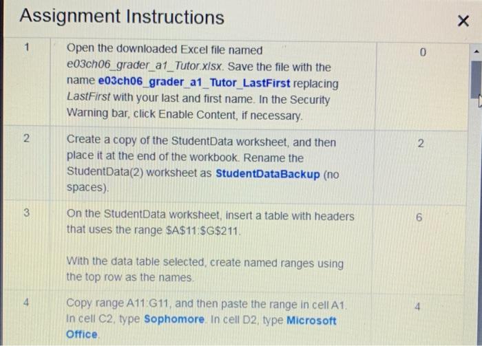

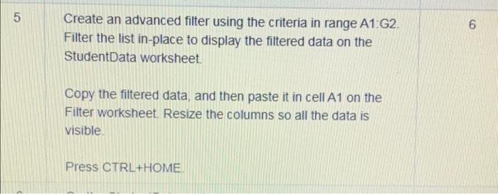
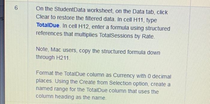
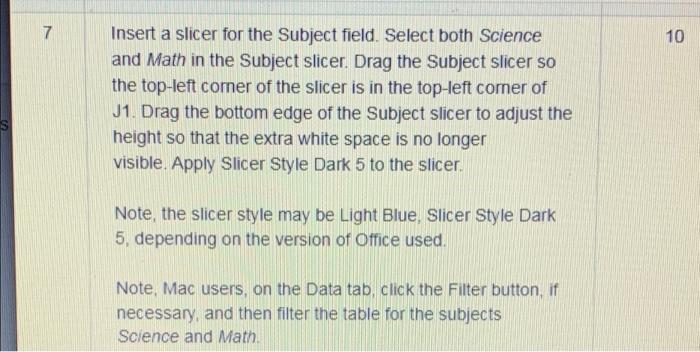
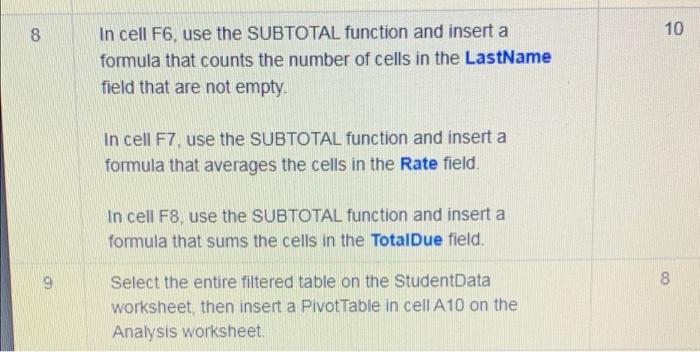
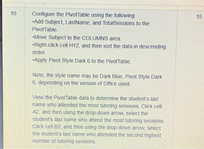
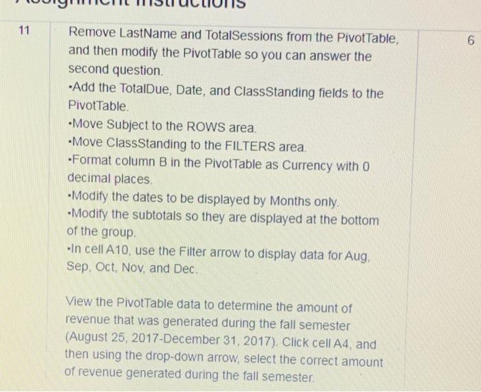
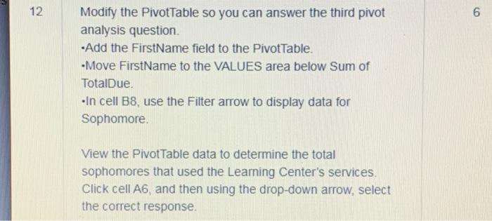
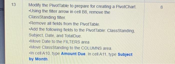
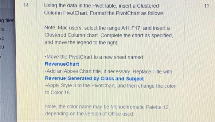
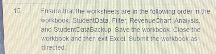
Assignment Instructions 1 0 Open the downloaded Excel file named e03ch06_grader_a1_Tutor.xlsx. Save the file with the name e03ch06_grader_a1_Tutor_LastFirst replacing LastFirst with your last and first name. In the Security Warning bar, click Enable Content, if necessary. 2 N 2. Create a copy of the StudentData worksheet, and then place it at the end of the workbook. Rename the StudentData(2) worksheet as StudentDataBackup (no spaces) 3 On the StudentData worksheet, insert a table with headers that uses the range $A$11:$G$211. 6 With the data table selected, create named ranges using the top row as the names 4 4 Copy range A11 G11, and then paste the range in cell A1 In cell C2, type Sophomore. In cell D2, type Microsoft Office 5 02 6 Create an advanced filter using the criteria in range A1 G2. Filter the list in-place to display the filtered data on the StudentData worksheet. Copy the filtered data, and then paste it in cell A1 on the Filter worksheet. Resize the columns so all the data is visible Press CTRL+HOME, 6 'S On the StudentData worksheet, on the Data tab, click Clear to restore the filtered data. In cell H11, type TotalDue. In cell H12, enter a formula using structured references that multiplies TotalSessions by Rate. Note, Mac users, copy the structured formula down through H211 Format the TotalDue column as Currency with 0 decimal places. Using the Create from Selection option, create a named range for the TotalDue column that uses the column heading as the name 7 10 Insert a slicer for the Subject field. Select both Science and Math in the Subject slicer. Drag the Subject slicer so the top-left corner of the slicer is in the top-left comer of J1. Drag the bottom edge of the Subject slicer to adjust the height so that the extra white space is no longer visible. Apply Slicer Style Dark 5 to the slicer. Note, the slicer style may be Light Blue, Slicer Style Dark 5, depending on the version of Office used. Note, Mac users, on the Data tab, click the Filter button if necessary, and then filter the table for the subjects Science and Math 8 10 In cell F6, use the SUBTOTAL function and insert a formula that counts the number of cells in the LastName field that are not empty. In cell F7, use the SUBTOTAL function and insert a formula that averages the cells in the Rate field. In cell F8, use the SUBTOTAL function and insert a formula that sums the cells in the TotalDue field. 9 8 Select the entire filtered table on the StudentData worksheet, then insert a Pivot Table in cell A10 on the Analysis worksheet. 10 15 Configure the PivotTable using the following: Add Subject, LastName, and TotalSessions to the Pivot Table. -Move Subject to the COLUMNS area. -Right-click cell H12, and then sort the data in descending order. -Apply Pivot Style Dark 6 to the PivotTable. Note the style name may be Dark Blue, Pivot Style Dark 6. depending on the version of Office used. View the Pivot Table data to determine the student's last name who attended the most tutoring sessions. Click cell A2, and then using the drop-down arrow, select the student's last name who attend the most tutoring sessions. Click cell B2 and then using the drop-down arrow, select the student's last name who attended the second highest number of tutoring sessions 11 6 Remove LastName and TotalSessions from the Pivot Table, and then modify the Pivot Table so you can answer the second question Add the TotalDue, Date, and Class Standing fields to the Pivot Table Move Subject to the ROWS area. -Move Class Standing to the FILTERS area. Format column B in the Pivot Table as Currency with 0 decimal places -Modify the dates to be displayed by Months only. Modify the subtotals so they are displayed at the bottom of the group .In cell A10, use the Filter arrow to display data for Aug, Sep Oct Nov, and Dec. View the Pivot Table data to determine the amount of revenue that was generated during the fall semester (August 25, 2017-December 31, 2017). Click cell A4, and then using the drop-down arrow, select the correct amount of revenue generated during the fall semester 12 6 Modify the PivotTable so you can answer the third pivot analysis question Add the FirstName field to the Pivot Table. -Move FirstName to the VALUES area below Sum of TotalDue. - In cell B8, use the Filter arrow to display data for Sophomore. View the Pivot Table data to determine the total sophomores that used the Learning Center's services. Click cell A6, and then using the drop-down arrow, select the correct response. 13 00 8 es Modify the PivotTable to prepare for creating a PivotChart. Using the filter arrow in cell B8, remove the ClassStanding filter -Remove all fields from the PivotTable. -Add the following fields to the PivotTable: ClassStanding, Subject Date and TotalDue. -Move Date to the FILTERS area -Move ClassStanding to the COLUMNS area. -In cell A10, type Amount Due. In cell A11, type Subject by Month 14 11 Using the data in the PivotTable, insert a Clustered Column PivotChart. Format the PivotChart as follows. ng files is 50 bu Note Mac users, select the range A11:F17. and insert a Clustered Column chart Complete the chart as specified, and move the legend to the right. -Move the PivotChart to a new sheet named RevenueChart - Add an Above Chart title, if necessary. Replace Title with Revenue Generated by Class and Subject Apply Style 8 to the PivotChart, and then change the color to Color 16 Note, the color name may be Monochromatic Palette 12, depending on the version of Office used. 15 Ensure that the worksheets are in the following order in the workbook. StudentData, Filter. RevenueChart Analysis, and StudentDataBackup. Save the workbook. Close the workbook and then exit Excel. Submit the workbook as directed Assignment Instructions 1 0 Open the downloaded Excel file named e03ch06_grader_a1_Tutor.xlsx. Save the file with the name e03ch06_grader_a1_Tutor_LastFirst replacing LastFirst with your last and first name. In the Security Warning bar, click Enable Content, if necessary. 2 N 2. Create a copy of the StudentData worksheet, and then place it at the end of the workbook. Rename the StudentData(2) worksheet as StudentDataBackup (no spaces) 3 On the StudentData worksheet, insert a table with headers that uses the range $A$11:$G$211. 6 With the data table selected, create named ranges using the top row as the names 4 4 Copy range A11 G11, and then paste the range in cell A1 In cell C2, type Sophomore. In cell D2, type Microsoft Office 5 02 6 Create an advanced filter using the criteria in range A1 G2. Filter the list in-place to display the filtered data on the StudentData worksheet. Copy the filtered data, and then paste it in cell A1 on the Filter worksheet. Resize the columns so all the data is visible Press CTRL+HOME, 6 'S On the StudentData worksheet, on the Data tab, click Clear to restore the filtered data. In cell H11, type TotalDue. In cell H12, enter a formula using structured references that multiplies TotalSessions by Rate. Note, Mac users, copy the structured formula down through H211 Format the TotalDue column as Currency with 0 decimal places. Using the Create from Selection option, create a named range for the TotalDue column that uses the column heading as the name 7 10 Insert a slicer for the Subject field. Select both Science and Math in the Subject slicer. Drag the Subject slicer so the top-left corner of the slicer is in the top-left comer of J1. Drag the bottom edge of the Subject slicer to adjust the height so that the extra white space is no longer visible. Apply Slicer Style Dark 5 to the slicer. Note, the slicer style may be Light Blue, Slicer Style Dark 5, depending on the version of Office used. Note, Mac users, on the Data tab, click the Filter button if necessary, and then filter the table for the subjects Science and Math 8 10 In cell F6, use the SUBTOTAL function and insert a formula that counts the number of cells in the LastName field that are not empty. In cell F7, use the SUBTOTAL function and insert a formula that averages the cells in the Rate field. In cell F8, use the SUBTOTAL function and insert a formula that sums the cells in the TotalDue field. 9 8 Select the entire filtered table on the StudentData worksheet, then insert a Pivot Table in cell A10 on the Analysis worksheet. 10 15 Configure the PivotTable using the following: Add Subject, LastName, and TotalSessions to the Pivot Table. -Move Subject to the COLUMNS area. -Right-click cell H12, and then sort the data in descending order. -Apply Pivot Style Dark 6 to the PivotTable. Note the style name may be Dark Blue, Pivot Style Dark 6. depending on the version of Office used. View the Pivot Table data to determine the student's last name who attended the most tutoring sessions. Click cell A2, and then using the drop-down arrow, select the student's last name who attend the most tutoring sessions. Click cell B2 and then using the drop-down arrow, select the student's last name who attended the second highest number of tutoring sessions 11 6 Remove LastName and TotalSessions from the Pivot Table, and then modify the Pivot Table so you can answer the second question Add the TotalDue, Date, and Class Standing fields to the Pivot Table Move Subject to the ROWS area. -Move Class Standing to the FILTERS area. Format column B in the Pivot Table as Currency with 0 decimal places -Modify the dates to be displayed by Months only. Modify the subtotals so they are displayed at the bottom of the group .In cell A10, use the Filter arrow to display data for Aug, Sep Oct Nov, and Dec. View the Pivot Table data to determine the amount of revenue that was generated during the fall semester (August 25, 2017-December 31, 2017). Click cell A4, and then using the drop-down arrow, select the correct amount of revenue generated during the fall semester 12 6 Modify the PivotTable so you can answer the third pivot analysis question Add the FirstName field to the Pivot Table. -Move FirstName to the VALUES area below Sum of TotalDue. - In cell B8, use the Filter arrow to display data for Sophomore. View the Pivot Table data to determine the total sophomores that used the Learning Center's services. Click cell A6, and then using the drop-down arrow, select the correct response. 13 00 8 es Modify the PivotTable to prepare for creating a PivotChart. Using the filter arrow in cell B8, remove the ClassStanding filter -Remove all fields from the PivotTable. -Add the following fields to the PivotTable: ClassStanding, Subject Date and TotalDue. -Move Date to the FILTERS area -Move ClassStanding to the COLUMNS area. -In cell A10, type Amount Due. In cell A11, type Subject by Month 14 11 Using the data in the PivotTable, insert a Clustered Column PivotChart. Format the PivotChart as follows. ng files is 50 bu Note Mac users, select the range A11:F17. and insert a Clustered Column chart Complete the chart as specified, and move the legend to the right. -Move the PivotChart to a new sheet named RevenueChart - Add an Above Chart title, if necessary. Replace Title with Revenue Generated by Class and Subject Apply Style 8 to the PivotChart, and then change the color to Color 16 Note, the color name may be Monochromatic Palette 12, depending on the version of Office used. 15 Ensure that the worksheets are in the following order in the workbook. StudentData, Filter. RevenueChart Analysis, and StudentDataBackup. Save the workbook. Close the workbook and then exit Excel. Submit the workbook as directed