help with project pls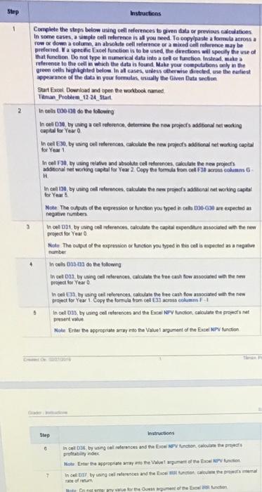

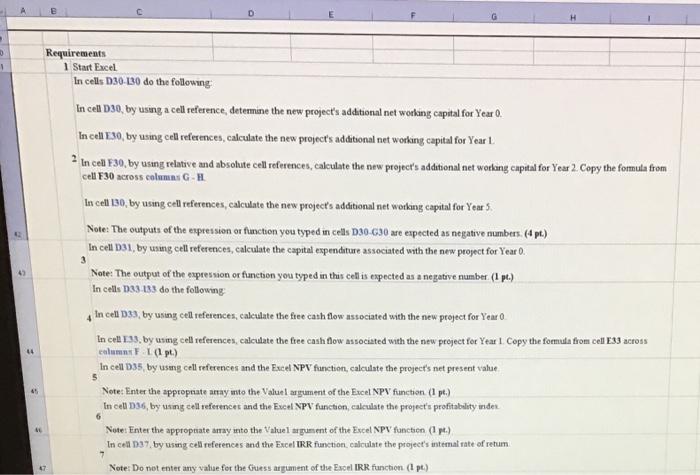
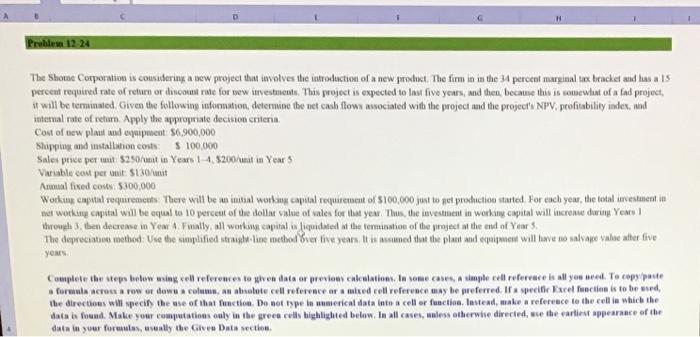
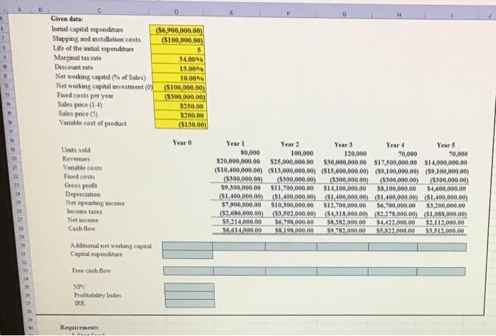
Step 1 2 Instructions Complete the steps below using cell references to given data or previous actions In some cases a simple cell reference is all you need to copy paste a forma across a row or down a colume, an absolute cell reference or a mixed cellere may be preferred a specific Exo function is to be used the erections will specify the use of that function. Do not type in numerical data into a color function. Instead, make reference to the cell in which the data is found. Make your computations only in the green cells inghighted below. In all cases, unless otherwise directed, use the rest appearance of the data in your formulas wally the Given Data con Surt Excel Download and open the workbook named Timan Problem 1224 Start In cells 000138 do the following In cell 030 byn a celi vederence, determine the new projects additional networking for Year Incel EX, by wsing cel references, calculate the new projects additional networking capital for Year 1 In cel F30, by using relative and absolute del references, calculate the new projects uditional mat working capital for Year 2 Copy the formula from cel F30 acros columns Incet 130by uning oil ruferences, takulate the new projects additional networking capital for Note: The outputs of the expression or function you typed in cel 030-030 are expected negative numbers In cel Das by using cleferences, caloutate the capital expenditult asociated with the new project for Year Nole. The output of the expression or function you typed in the cell as expected as a negative In cels 030-01 do the following In de 23 by using our reference calculate the true cash flow mounted with the sem for Year in cell en by using cell references, calculate the free cash flow associated with the new project for Year 1 Copy the formula from all around In cell 03, by using cell references and the BNP function, calculate the progeshet present value Mole Enter the appropriate any to the value argument of the Excel Pfunction > 5 Step Instructions 0 In cel by using career and the NPV anchonete profitabindex Home Enter the appropriate way to the Vermelho In all DT by se read the other oftum te Ouest mechon 1 Requirements 1 Start Excel In cells 130 130 do the following In celt 130, by using a cell reference, determine the new project's additional net working capital for Year 0. In cell E30, by using cell references, calculate the new project's additional net working capital for Year 1 2 In cell F30, by using relative and absolute cell references, calculate the new project's additional net working capital for Year 2. Copy the formula from cell F30 across columns GH In cell 130, by using cell references, calculate the new project's additional net working capital for Year 5 Note: The outputs of the expression or function you typed in cells D30G30 are expected as negative numbers. (dpi) In cell DS1, by using cell references, calculate the capital expenditure associated with the new project for Year 0. Note: The output of the expression or fianction you typed in this cell is expected as a negative number (1) In cells 033-133 do the following In cell 0.33, by using cell references, calculate the free cath flow associated with the new project for Year o In cell 133by using cell references, calculate the free cash flow associated with the new project for Year I. Copy the formula from cell E33 across columns 1 (1) In cell 035, by using cell references and the Excel NPV function, calculate the project's not present value Note: Enter the appropriate aray unto the Valuel argument of the Excel NPV function (1 p.) In cell 036, by using cell references and the Excel NPV function, calculate the project's profitability under Note: Enter the appropriate amay into the Valuel argument of the Excel NPV function (1 p.) In cell D37, by using cell references and the Excel IRR function calculate the project's internal rate of retum 3 5 45 6 Note: Do not enter any valae for the Guess argument of the Excel IRR function (pt) Problem 12. 24 The Shome Corporation is considering a new project that involves the introduction of a new product. The firm in in the 34 percent marginal tax bracket and has als percent required rate of return or discount rate for new investments. This project is expected to Inut five years, and then because this is somewhat of a fad project, it will be terminated. Given the following information, determine the net cash flow associated with the project and the project's NPV, profitability index, and internal rate of return. Apply the appropriate decision criteria Cost of now plaust and equipment. 56.900,000 Shipping and installation code $ 100.000 Sales price per it $250/mit in Years 1-4, 5200/unit in Year 5 Variable cost per uut 130/unit Anal fixed costs $300,000 Working capital requirements . There will be an initial working capital tequirement of $100,000 just to get production started. For each year, the total investment in wat working capital will be equal to 10 percent of the della value of sales for that year. Thus, the investment in working capital will increme during Years through then decrease m Year A Fally all working capital s fiquidated at the termination of the project at the end of Years The depreciation method: Use the simplified straighie method ver five years. It is somed that the plant and equipment will have to salvape valocater five years Complete the steps below using well references to them at or previous calculations. In some cases, A simple el refervace ke all you need to copy paste formula acou a row or down colum, an absolute cell reference or a mixed cell reference may be preferred. If a specific Excel function is to be used the directions will specify the use of that function. Do not type in numerical data into a cell or function. Instead, make a reference to the cell in which the data is found. Make your computations only in the green cells highlighted below. In all cases, unless otherwise directed, use the earliest appearance of the data in your formas, wally the Give Data section 7 Given data: Initial capital expenditure ($6,900,000.00) Shopping and installation costs ($100,000.00) Life of the initial expenditure 5 Marginal tax rate 34.00% Discount rate 15.0096 Networking capital of Sales) 10.0096 Net working capital investment (O) ($100,000.00) Fured costs per year 18300,000.00) Sales pnce (14) $250.00 Sales price (5) $200.00 Variable cost of product (5130.00) 11 Year 0 Units sold Revenues Vanable costs Fued costs Gross profit Depreciation Netopearing income Income taxes Net income Cash flow Year 1 Year 2 Year 3 Year 4 Year 5 80,000 100,000 120,000 70,000 70,000 $20,000,000.00 $25,000,000.00 $30,000,000.00 $17.500,000.00 $14,000,000.00 ($10,400,000.00) ($13,000,000,00) (815,600,000.00) (59,100,000,00) (59,100,000.00) (8300,000.00) ($300,000.00) ($300,000.00) ($100,000.00) ($300,000.00) 59,100,000.00 $11.700,000.00 $14.100,000.00 58,100,000.00 $4,600,000.00 ($1,400,000.00 ($1,400,000.00) ($1,400,000.00) ($1,400,000.00) ($1,400,000,00) $7.900,000.00 $10,300,000.00 $12,700,000.00 $6,700,000.00 53,200,000.00 ($2,686,000.00) ($3,502,000.00) ($4,318,000,00){$2,278,000.00) ($1,088,000.00) $5,214,000.00 $6,798,000.00 $8.382,000.00 $4,422,000.00 $2,112,000.00 $6,614,000.00 S8,198,000.00 $9.782,000.00 $5822,000.00 $1,312,000.00 Additional cut working capital Capital expenditure Free cash flow 14 NPV Profitabdary Index IRR 40 Requirements Step 1 2 Instructions Complete the steps below using cell references to given data or previous actions In some cases a simple cell reference is all you need to copy paste a forma across a row or down a colume, an absolute cell reference or a mixed cellere may be preferred a specific Exo function is to be used the erections will specify the use of that function. Do not type in numerical data into a color function. Instead, make reference to the cell in which the data is found. Make your computations only in the green cells inghighted below. In all cases, unless otherwise directed, use the rest appearance of the data in your formulas wally the Given Data con Surt Excel Download and open the workbook named Timan Problem 1224 Start In cells 000138 do the following In cell 030 byn a celi vederence, determine the new projects additional networking for Year Incel EX, by wsing cel references, calculate the new projects additional networking capital for Year 1 In cel F30, by using relative and absolute del references, calculate the new projects uditional mat working capital for Year 2 Copy the formula from cel F30 acros columns Incet 130by uning oil ruferences, takulate the new projects additional networking capital for Note: The outputs of the expression or function you typed in cel 030-030 are expected negative numbers In cel Das by using cleferences, caloutate the capital expenditult asociated with the new project for Year Nole. The output of the expression or function you typed in the cell as expected as a negative In cels 030-01 do the following In de 23 by using our reference calculate the true cash flow mounted with the sem for Year in cell en by using cell references, calculate the free cash flow associated with the new project for Year 1 Copy the formula from all around In cell 03, by using cell references and the BNP function, calculate the progeshet present value Mole Enter the appropriate any to the value argument of the Excel Pfunction > 5 Step Instructions 0 In cel by using career and the NPV anchonete profitabindex Home Enter the appropriate way to the Vermelho In all DT by se read the other oftum te Ouest mechon 1 Requirements 1 Start Excel In cells 130 130 do the following In celt 130, by using a cell reference, determine the new project's additional net working capital for Year 0. In cell E30, by using cell references, calculate the new project's additional net working capital for Year 1 2 In cell F30, by using relative and absolute cell references, calculate the new project's additional net working capital for Year 2. Copy the formula from cell F30 across columns GH In cell 130, by using cell references, calculate the new project's additional net working capital for Year 5 Note: The outputs of the expression or function you typed in cells D30G30 are expected as negative numbers. (dpi) In cell DS1, by using cell references, calculate the capital expenditure associated with the new project for Year 0. Note: The output of the expression or fianction you typed in this cell is expected as a negative number (1) In cells 033-133 do the following In cell 0.33, by using cell references, calculate the free cath flow associated with the new project for Year o In cell 133by using cell references, calculate the free cash flow associated with the new project for Year I. Copy the formula from cell E33 across columns 1 (1) In cell 035, by using cell references and the Excel NPV function, calculate the project's not present value Note: Enter the appropriate aray unto the Valuel argument of the Excel NPV function (1 p.) In cell 036, by using cell references and the Excel NPV function, calculate the project's profitability under Note: Enter the appropriate amay into the Valuel argument of the Excel NPV function (1 p.) In cell D37, by using cell references and the Excel IRR function calculate the project's internal rate of retum 3 5 45 6 Note: Do not enter any valae for the Guess argument of the Excel IRR function (pt) Problem 12. 24 The Shome Corporation is considering a new project that involves the introduction of a new product. The firm in in the 34 percent marginal tax bracket and has als percent required rate of return or discount rate for new investments. This project is expected to Inut five years, and then because this is somewhat of a fad project, it will be terminated. Given the following information, determine the net cash flow associated with the project and the project's NPV, profitability index, and internal rate of return. Apply the appropriate decision criteria Cost of now plaust and equipment. 56.900,000 Shipping and installation code $ 100.000 Sales price per it $250/mit in Years 1-4, 5200/unit in Year 5 Variable cost per uut 130/unit Anal fixed costs $300,000 Working capital requirements . There will be an initial working capital tequirement of $100,000 just to get production started. For each year, the total investment in wat working capital will be equal to 10 percent of the della value of sales for that year. Thus, the investment in working capital will increme during Years through then decrease m Year A Fally all working capital s fiquidated at the termination of the project at the end of Years The depreciation method: Use the simplified straighie method ver five years. It is somed that the plant and equipment will have to salvape valocater five years Complete the steps below using well references to them at or previous calculations. In some cases, A simple el refervace ke all you need to copy paste formula acou a row or down colum, an absolute cell reference or a mixed cell reference may be preferred. If a specific Excel function is to be used the directions will specify the use of that function. Do not type in numerical data into a cell or function. Instead, make a reference to the cell in which the data is found. Make your computations only in the green cells highlighted below. In all cases, unless otherwise directed, use the earliest appearance of the data in your formas, wally the Give Data section 7 Given data: Initial capital expenditure ($6,900,000.00) Shopping and installation costs ($100,000.00) Life of the initial expenditure 5 Marginal tax rate 34.00% Discount rate 15.0096 Networking capital of Sales) 10.0096 Net working capital investment (O) ($100,000.00) Fured costs per year 18300,000.00) Sales pnce (14) $250.00 Sales price (5) $200.00 Variable cost of product (5130.00) 11 Year 0 Units sold Revenues Vanable costs Fued costs Gross profit Depreciation Netopearing income Income taxes Net income Cash flow Year 1 Year 2 Year 3 Year 4 Year 5 80,000 100,000 120,000 70,000 70,000 $20,000,000.00 $25,000,000.00 $30,000,000.00 $17.500,000.00 $14,000,000.00 ($10,400,000.00) ($13,000,000,00) (815,600,000.00) (59,100,000,00) (59,100,000.00) (8300,000.00) ($300,000.00) ($300,000.00) ($100,000.00) ($300,000.00) 59,100,000.00 $11.700,000.00 $14.100,000.00 58,100,000.00 $4,600,000.00 ($1,400,000.00 ($1,400,000.00) ($1,400,000.00) ($1,400,000.00) ($1,400,000,00) $7.900,000.00 $10,300,000.00 $12,700,000.00 $6,700,000.00 53,200,000.00 ($2,686,000.00) ($3,502,000.00) ($4,318,000,00){$2,278,000.00) ($1,088,000.00) $5,214,000.00 $6,798,000.00 $8.382,000.00 $4,422,000.00 $2,112,000.00 $6,614,000.00 S8,198,000.00 $9.782,000.00 $5822,000.00 $1,312,000.00 Additional cut working capital Capital expenditure Free cash flow 14 NPV Profitabdary Index IRR 40 Requirements