Here is a link to the Excel file on Google Sheets: https://docs.google.com/spreadsheets/d/1UMAQayMJJr6VZcmhkJqoBlQutqGUoakNP0HYfgTTbvg/edit?usp=sharing

Please save the file as an Excel document and open it in Excel. Please post Excel screenshots of your solution once you figured it out. Thank you!

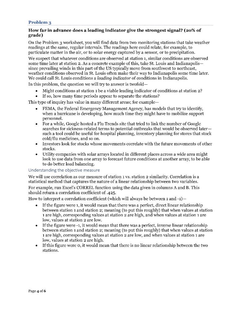
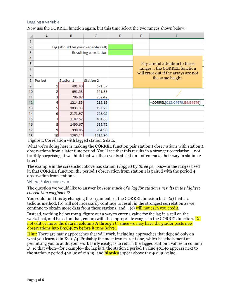
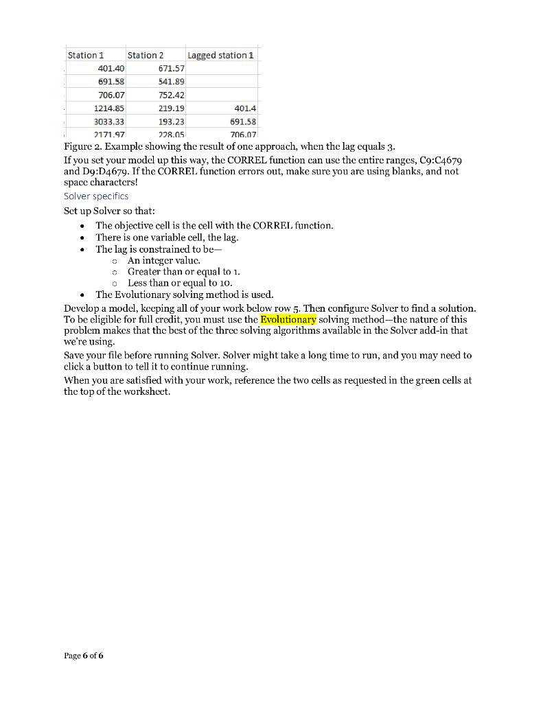
Problem 3 How far in advance does a leading indicator give the strongest signal? (20% of grade) On the Problem 3 worksheet, you will find data from two monitoring stations that take weather readings at the same, regular intervals. The readings here could relate, for example, to particulate matter in the air, or to solar energy captured by a sensor, or to precipitation. We suspect that whatever conditions are observed at station 1, similar conditions are observed some time later at station 2. As a concrete example of this, take St. Louis and Indianapolis- since prevailing winds in this part of the US typically move from southwest to northcast, weather conditions observed in St. Louis often make their way to Indianapolis some time later. We could call St. Louis conditions a leading indicator of conditions in Indianapolis. In this problem, the question we will try to answer is twofold- Might conditions at station 1 be a viable leading indicator of conditions at station 2? If so, how many time periods appear to separate the stations? This type of inquiry has value in many different areas; for example- FEMA, the Federal Emergency Management Agency, has models that try to identify, when a hurricane is developing, how much time they might have to mobilize support personnel. For a while, Googlc hosted a Flu Trends site that tricd to link the number of Google searches for sickness-related terms to potential outbreaks that would be observed later- such a tool could be useful for hospital planning, inventory planning for stores that stock cold/flu medicines, and so on. Investors look for stocks whose movements correlate with the future movements of other stocks. Utility companies with solar arrays located in different places across a wide area might look to use data from one array to forecast future conditions at another array, to be able to do better load balancing. Understanding the objective measure We will use correlation as our measure of station 1 vs. station 2 similarity. Correlation is a statistical method that captures the nature of a linear relationship between two variables. For example, run Excel's CORREL function using the data given in columns A and B. This should return a correlation coefficient of .425. How to interpret a correlation coefficient (which will always be between 1 and -1)- If the figure were 1, it would mean that there was a perfect, direct linear relationship between station 1 and station 2; meaning (to put this roughly) that when values at station 1 are high, corresponding values at station 2 are high, and when values at station 1 are low, values at station 2 are low. If the figure were -1, it would mean that there was a perfect, inverse linear relationship between station 1 and station 2; meaning (to put this roughly) that when values at station are high, corresponding values at station 2 are low, and when values at station i are low, values at station 2 are high. If this figure were o, it would mean that there is no lincar relationship between the two stations. Page 4 of 6 Lagging a variable Now usc thc CORREL function again, but this time select the two ranges shown below: A B C D E 1 2 Lag (should be your variable cell) Resulting correlation 3 4 5 2 4 15 Pay careful attention to these 6 ranges... the CORREL function 7 will error out if the arrays are not the same height 8 Period Station 1 Station 2 9 401.40 671.57 10 691.58 541.89 11 3 706.07 752.42 12 1214.85 219.19 =CORREL(C12:04679,89:B4676) 13 5 3033.33 193.23 14 6 2171.97 228.05 7 1147.52 401.65 16 8 1490.67 689.72 17 9 998.06 704.901 18 10 1295.14 1215.901 Figure 1. Correlation with lagged station 2 data. What we're doing here is making the CORREL function pair station 1 observations with station 2 obscrvations from a later time period. You'll scc that this results in a stronger correlation... not terribly surprising, if we think that weather events at station 1 often make their way to station 2 later! The example in the screenshot above has station i lagged three periods-in the ranges used in that CORREL function, the period 1 observation from station 1 is paired with the period 4 observation from station 2. Where Solver comes in The question we would like to answer is: How much of a lag for station 1 results in the highest correlation coefficient? You could find this by changing the arguments of the CORREL function but-(a) that is a tedious method, (b) will not necessarily continue to result in the strongest correlation as we continuc to obtain more data from these stations, and... (c) will not carn you crcdit. Instead, working below row 5, figure out a way to enter a value for the lag in a ocll on the worksheet, and based on that, end up with the appropriate ranges in the CORREL function. Do not edit or move the data in columns A through C, since we may have the grader paste new observations into B9:C4679 before it runs Solver. Hint: There are many approaches that will work, including approaches that depend only on what you learned in K201/4. Probably the most transparent one, which has the benefit of permitting you to audit your work fairly easily, is to return the lagged station 1 values in column D, so that when-for example the lag is 3, the station 1 period 1 value 401.40 appears next to the station 2 period 4 value of 219.19, and blanks appear above the 401.40 value. Page 5 of 6 Station 1 Station 2 Lagged station 1 401.40 671.57 691.58 541.89 706.07 752.42 1214.85 219.19 401.4 3033.33 193.23 691.58 2171.97 228.05 706.07 Figure 2. Example showing the result of one approach, when the lag equals 3. If you set your model up this way, the CORREL function can use the entire ranges, C9:C4679 and D9:04679. If the CORREL function errors out, make sure you are using blanks, and not space characters! Solver specifics Set up Solver so that: The objective cell is the cell with the CORREL function. There is one variable cell, the lag. The lag is constrained to be- An integer valuc. o Greater than or equal to 1. o Less than or equal to 10. The Evolutionary solving method is used. Develop a model, keeping all of your work below row 5. Then configure Solver to find a solution. To be eligible for full credit, you must use the Evolutionary solving method-the nature of this problem makes that the best of the three solving algorithms available in the Solver add-in that We're using. Save your file before running Solver. Solver might take a long time to run, and you may need to click a button to tell it to continue running. When you are satisfied with your work, reference the two cells as requested in the green cells at the top of the worksheet. . Page 6 of 6 Problem 3 How far in advance does a leading indicator give the strongest signal? (20% of grade) On the Problem 3 worksheet, you will find data from two monitoring stations that take weather readings at the same, regular intervals. The readings here could relate, for example, to particulate matter in the air, or to solar energy captured by a sensor, or to precipitation. We suspect that whatever conditions are observed at station 1, similar conditions are observed some time later at station 2. As a concrete example of this, take St. Louis and Indianapolis- since prevailing winds in this part of the US typically move from southwest to northcast, weather conditions observed in St. Louis often make their way to Indianapolis some time later. We could call St. Louis conditions a leading indicator of conditions in Indianapolis. In this problem, the question we will try to answer is twofold- Might conditions at station 1 be a viable leading indicator of conditions at station 2? If so, how many time periods appear to separate the stations? This type of inquiry has value in many different areas; for example- FEMA, the Federal Emergency Management Agency, has models that try to identify, when a hurricane is developing, how much time they might have to mobilize support personnel. For a while, Googlc hosted a Flu Trends site that tricd to link the number of Google searches for sickness-related terms to potential outbreaks that would be observed later- such a tool could be useful for hospital planning, inventory planning for stores that stock cold/flu medicines, and so on. Investors look for stocks whose movements correlate with the future movements of other stocks. Utility companies with solar arrays located in different places across a wide area might look to use data from one array to forecast future conditions at another array, to be able to do better load balancing. Understanding the objective measure We will use correlation as our measure of station 1 vs. station 2 similarity. Correlation is a statistical method that captures the nature of a linear relationship between two variables. For example, run Excel's CORREL function using the data given in columns A and B. This should return a correlation coefficient of .425. How to interpret a correlation coefficient (which will always be between 1 and -1)- If the figure were 1, it would mean that there was a perfect, direct linear relationship between station 1 and station 2; meaning (to put this roughly) that when values at station 1 are high, corresponding values at station 2 are high, and when values at station 1 are low, values at station 2 are low. If the figure were -1, it would mean that there was a perfect, inverse linear relationship between station 1 and station 2; meaning (to put this roughly) that when values at station are high, corresponding values at station 2 are low, and when values at station i are low, values at station 2 are high. If this figure were o, it would mean that there is no lincar relationship between the two stations. Page 4 of 6 Lagging a variable Now usc thc CORREL function again, but this time select the two ranges shown below: A B C D E 1 2 Lag (should be your variable cell) Resulting correlation 3 4 5 2 4 15 Pay careful attention to these 6 ranges... the CORREL function 7 will error out if the arrays are not the same height 8 Period Station 1 Station 2 9 401.40 671.57 10 691.58 541.89 11 3 706.07 752.42 12 1214.85 219.19 =CORREL(C12:04679,89:B4676) 13 5 3033.33 193.23 14 6 2171.97 228.05 7 1147.52 401.65 16 8 1490.67 689.72 17 9 998.06 704.901 18 10 1295.14 1215.901 Figure 1. Correlation with lagged station 2 data. What we're doing here is making the CORREL function pair station 1 observations with station 2 obscrvations from a later time period. You'll scc that this results in a stronger correlation... not terribly surprising, if we think that weather events at station 1 often make their way to station 2 later! The example in the screenshot above has station i lagged three periods-in the ranges used in that CORREL function, the period 1 observation from station 1 is paired with the period 4 observation from station 2. Where Solver comes in The question we would like to answer is: How much of a lag for station 1 results in the highest correlation coefficient? You could find this by changing the arguments of the CORREL function but-(a) that is a tedious method, (b) will not necessarily continue to result in the strongest correlation as we continuc to obtain more data from these stations, and... (c) will not carn you crcdit. Instead, working below row 5, figure out a way to enter a value for the lag in a ocll on the worksheet, and based on that, end up with the appropriate ranges in the CORREL function. Do not edit or move the data in columns A through C, since we may have the grader paste new observations into B9:C4679 before it runs Solver. Hint: There are many approaches that will work, including approaches that depend only on what you learned in K201/4. Probably the most transparent one, which has the benefit of permitting you to audit your work fairly easily, is to return the lagged station 1 values in column D, so that when-for example the lag is 3, the station 1 period 1 value 401.40 appears next to the station 2 period 4 value of 219.19, and blanks appear above the 401.40 value. Page 5 of 6 Station 1 Station 2 Lagged station 1 401.40 671.57 691.58 541.89 706.07 752.42 1214.85 219.19 401.4 3033.33 193.23 691.58 2171.97 228.05 706.07 Figure 2. Example showing the result of one approach, when the lag equals 3. If you set your model up this way, the CORREL function can use the entire ranges, C9:C4679 and D9:04679. If the CORREL function errors out, make sure you are using blanks, and not space characters! Solver specifics Set up Solver so that: The objective cell is the cell with the CORREL function. There is one variable cell, the lag. The lag is constrained to be- An integer valuc. o Greater than or equal to 1. o Less than or equal to 10. The Evolutionary solving method is used. Develop a model, keeping all of your work below row 5. Then configure Solver to find a solution. To be eligible for full credit, you must use the Evolutionary solving method-the nature of this problem makes that the best of the three solving algorithms available in the Solver add-in that We're using. Save your file before running Solver. Solver might take a long time to run, and you may need to click a button to tell it to continue running. When you are satisfied with your work, reference the two cells as requested in the green cells at the top of the worksheet. . Page 6 of 6