Here is what I have so far.
#include #include #include
using namespace std;
struct Weibull { double alpha; double beta; double meanResult; Weibull(); ~Weibull (); void Density (Weibull, Weibull); void Mean (double, double); void displayResults (Weibull, Weibull); };
Weibull::Weibull() { //constructor this -> alpha = 0; this -> beta = 0; this -> meanResult = 0; }
Weibull::~Weibull() { //destructor }
void Weibull::Density(Weibull distribution2, Weibull distribution3) { }
void Weibull::Mean(double aplha, double beta) { this -> alpha = alpha; this -> beta = beta; this -> meanResult = beta*(tgamma(1+1/alpha)); }
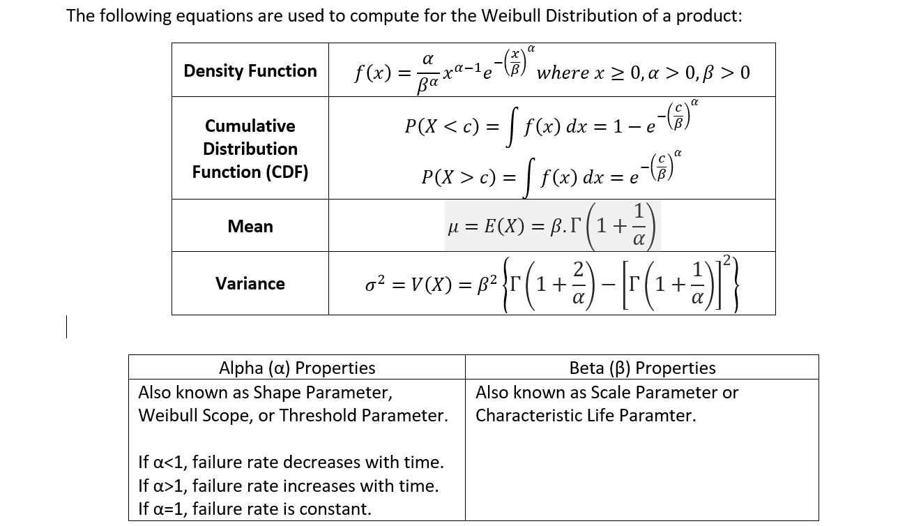
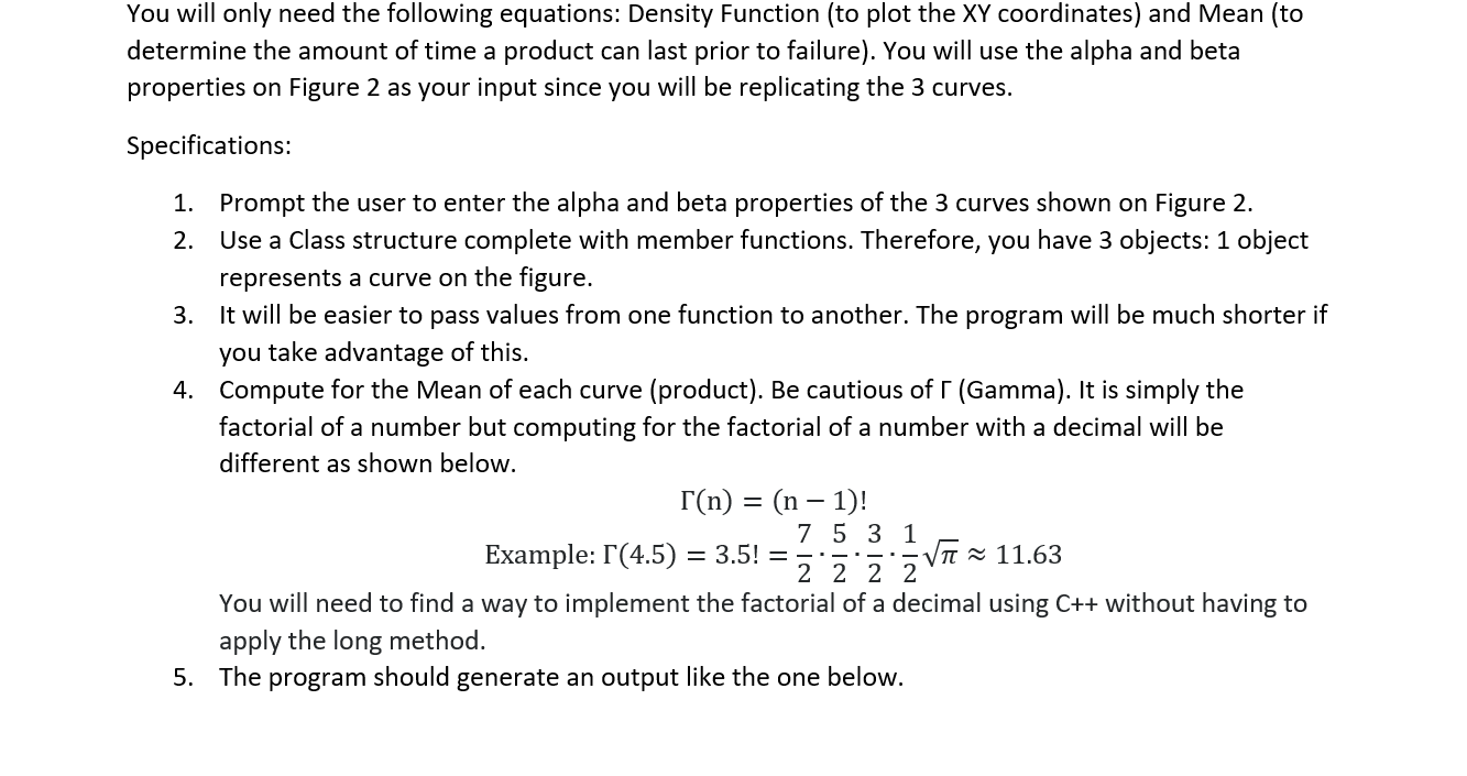
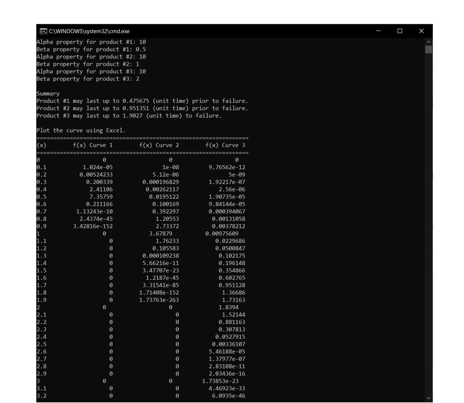
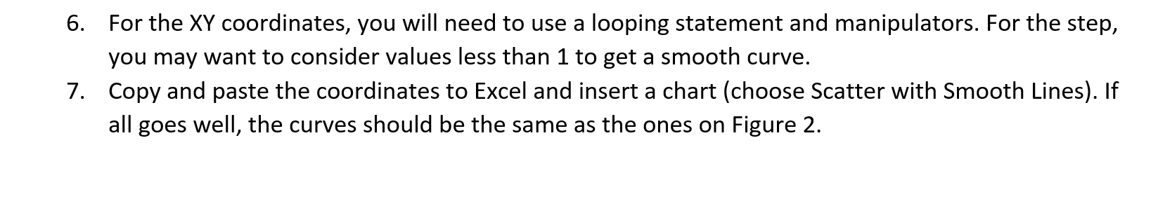
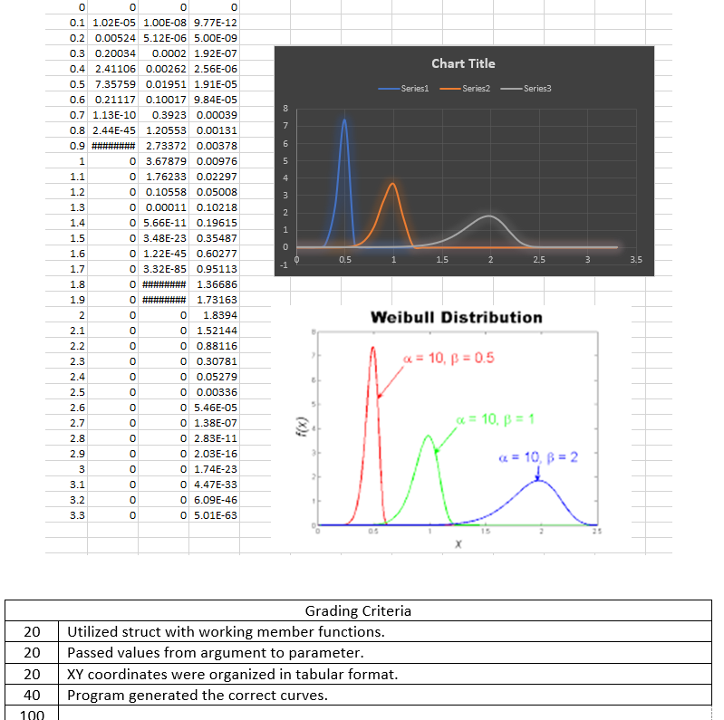
void Weibull::displayResults(Weibull distribution2, Weibull distribution3) { cout The following equations are used to compute for the Weibull Distribution of a product: Density Function f(x) = Cumulative Distribution Function (CDF) - na parte-Owhere x 2 0,a > 0,8 > 0 P(X c) = f(x) dx = e --C) u = E(X) = p.1(1+) 22-W63)-3(3+3(+2) Mean Variance Alpha (a) Properties Also known as Shape Parameter, Weibull Scope, or Threshold Parameter. Beta () Properties Also known as Scale Parameter or Characteristic Life Paramter. If a1, failure rate increases with time. If a=1, failure rate is constant. You will only need the following equations: Density Function (to plot the XY coordinates) and Mean (to determine the amount of time a product can last prior to failure). You will use the alpha and beta properties on Figure 2 as your input since you will be replicating the 3 curves. Specifications: 1. Prompt the user to enter the alpha and beta properties of the 3 curves shown on Figure 2. 2. Use a Class structure complete with member functions. Therefore, you have 3 objects: 1 object represents a curve on the figure. 3. It will be easier to pass values from one function to another. The program will be much shorter if you take advantage of this. 4. Compute for the Mean of each curve (product). Be cautious of F (Gamma). It is simply the factorial of a number but computing for the factorial of a number with a decimal will be different as shown below. T(n) = (n - 1)! 7 5 3 1 Example: T(4.5) = 3.5! = T 11.63 2 2 2 2 You will need to find a way to implement the factorial of a decimal using C++ without having to apply the long method. 5. The program should generate an output like the one below. C. C:\WINDOWS\system32\cmd.exe Alpha property for product #1: 10 Beta property for product #1: 0.5 Alpha property for product #2: 10 Beta property for product #2: 1 Alpha property for product #3: 10 Beta property for product #3: 2 Summary Product #1 may last up to 0.475675 (unit time) prior to failure. Product #2 may last up to 0.951351 (unit time) prior to failure. Product #3 may last up to 1.9027 (unit time) to failure. Plot the curve using Excel. f(x) Curve 1 f(x) Curve 2 f(x) Curve 3 1.024e-65 0.00524233 0.200339 2.41106 7.35759 0.211166 1.13243e-10 2.4374e-45 3.42816e-152 @ 1e-08 5.12e-06 0.000196829 0.00262117 0.0195122 0.100169 0.392297 1.20553 2.73372 3.67879 1.76233 0.105583 0.000109238 5.66216e-11 3.47707e-23 1.2187e-45 3.31541e-85 1.71408e-152 1.73763e-263 0 0.1 9.2 0.3 0.4 0.5 0.6 0.7 0.8 0.9 1 1.1 1.2 1.3 1.4 1.5 1.6 1.7 1.8 1.9 2 2.1 2.2 2.3 2.4 2.5 2.6 2.7 2.8 2.9 3 3.1 3.2 0 9.76562e-12 5e-29 1.92217e-07 2.56e-06 1.90735e-05 9.84144e-05 0.000394067 0.00131058 0.00378212 0.00975609 0.0229686 0.0500847 0.102175 0.196148 0.354866 0.602765 0.951128 1.36686 1.73163 1.8394 1.52144 0.881163 0.307813 0.0527915 0.00336107 5.46188e-05 1.37977e-07 2.83108e-11 2.03436e-16 1.73853e-23 4.46923e-33 6.0935e-46 0 0 @ @ 0 6. For the XY coordinates, you will need to use a looping statement and manipulators. For the step, you may want to consider values less than 1 to get a smooth curve. 7. Copy and paste the coordinates to Excel and insert a chart (choose Scatter with Smooth Lines). If all goes well, the curves should be the same as the ones on Figure 2. Chart Title Series1 Series2 Series3 7 6 5 4 3 2 1 1.5 0 0 0 0 0 0.1 1.02E-05 1.00E-08 9.77E-12 0.2 0.00524 5.12E-06 5.00E-09 0.3 0.20034 0.0002 1.92E-07 0.4 2.41106 0.00262 2.56E-06 0.5 7.35759 0.01951 1.91E-05 0.6 0.21117 0.10017 9.84E-05 0.7 1.13E-10 0.3923 0.00039 0.8 2.44E-45 1.20553 0.00131 0.9 ######## 2.73372 0.00378 1 0 3.67879 0.00976 1.1 0 1.76233 0.02297 1.2 0 0.10558 0.05008 1.3 0 0.00011 0.10218 1.4 0 5.66E-11 0.19615 0 3.48E-23 0.35487 1.6 0 1.22E-45 0.60277 1.7 0 3.32E-85 0.95113 1.8 1.36686 1.9 0 ######## 1.73163 2 0 1.8394 2.1 0 1.52144 2.2 0 0.88116 2.3 0 0.30781 2.4 0 0.05279 2.5 0 0.00336 2.6 0 5.46E-05 2.7 0 1.38E-07 2.8 0 2.83E-11 2.9 0 02.03E-16 3 0 1.74E-23 3.1 0 0 4.47E-33 3.2 06.09E-46 3.3 0 05.01E-63 0.5 1.5 2.5 3 3.5 Weibull Distribution O O O O O O O O O O O O O O O OOOO a = 10, B = 0.5 a = 10. B = 1 = 10, B = 2 25 20 20 20 40 Grading Criteria Utilized struct with working member functions. Passed values from argument to parameter. XY coordinates were organized in tabular format. Program generated the correct curves. 100 The following equations are used to compute for the Weibull Distribution of a product: Density Function f(x) = Cumulative Distribution Function (CDF) - na parte-Owhere x 2 0,a > 0,8 > 0 P(X c) = f(x) dx = e --C) u = E(X) = p.1(1+) 22-W63)-3(3+3(+2) Mean Variance Alpha (a) Properties Also known as Shape Parameter, Weibull Scope, or Threshold Parameter. Beta () Properties Also known as Scale Parameter or Characteristic Life Paramter. If a1, failure rate increases with time. If a=1, failure rate is constant. You will only need the following equations: Density Function (to plot the XY coordinates) and Mean (to determine the amount of time a product can last prior to failure). You will use the alpha and beta properties on Figure 2 as your input since you will be replicating the 3 curves. Specifications: 1. Prompt the user to enter the alpha and beta properties of the 3 curves shown on Figure 2. 2. Use a Class structure complete with member functions. Therefore, you have 3 objects: 1 object represents a curve on the figure. 3. It will be easier to pass values from one function to another. The program will be much shorter if you take advantage of this. 4. Compute for the Mean of each curve (product). Be cautious of F (Gamma). It is simply the factorial of a number but computing for the factorial of a number with a decimal will be different as shown below. T(n) = (n - 1)! 7 5 3 1 Example: T(4.5) = 3.5! = T 11.63 2 2 2 2 You will need to find a way to implement the factorial of a decimal using C++ without having to apply the long method. 5. The program should generate an output like the one below. C. C:\WINDOWS\system32\cmd.exe Alpha property for product #1: 10 Beta property for product #1: 0.5 Alpha property for product #2: 10 Beta property for product #2: 1 Alpha property for product #3: 10 Beta property for product #3: 2 Summary Product #1 may last up to 0.475675 (unit time) prior to failure. Product #2 may last up to 0.951351 (unit time) prior to failure. Product #3 may last up to 1.9027 (unit time) to failure. Plot the curve using Excel. f(x) Curve 1 f(x) Curve 2 f(x) Curve 3 1.024e-65 0.00524233 0.200339 2.41106 7.35759 0.211166 1.13243e-10 2.4374e-45 3.42816e-152 @ 1e-08 5.12e-06 0.000196829 0.00262117 0.0195122 0.100169 0.392297 1.20553 2.73372 3.67879 1.76233 0.105583 0.000109238 5.66216e-11 3.47707e-23 1.2187e-45 3.31541e-85 1.71408e-152 1.73763e-263 0 0.1 9.2 0.3 0.4 0.5 0.6 0.7 0.8 0.9 1 1.1 1.2 1.3 1.4 1.5 1.6 1.7 1.8 1.9 2 2.1 2.2 2.3 2.4 2.5 2.6 2.7 2.8 2.9 3 3.1 3.2 0 9.76562e-12 5e-29 1.92217e-07 2.56e-06 1.90735e-05 9.84144e-05 0.000394067 0.00131058 0.00378212 0.00975609 0.0229686 0.0500847 0.102175 0.196148 0.354866 0.602765 0.951128 1.36686 1.73163 1.8394 1.52144 0.881163 0.307813 0.0527915 0.00336107 5.46188e-05 1.37977e-07 2.83108e-11 2.03436e-16 1.73853e-23 4.46923e-33 6.0935e-46 0 0 @ @ 0 6. For the XY coordinates, you will need to use a looping statement and manipulators. For the step, you may want to consider values less than 1 to get a smooth curve. 7. Copy and paste the coordinates to Excel and insert a chart (choose Scatter with Smooth Lines). If all goes well, the curves should be the same as the ones on Figure 2. Chart Title Series1 Series2 Series3 7 6 5 4 3 2 1 1.5 0 0 0 0 0 0.1 1.02E-05 1.00E-08 9.77E-12 0.2 0.00524 5.12E-06 5.00E-09 0.3 0.20034 0.0002 1.92E-07 0.4 2.41106 0.00262 2.56E-06 0.5 7.35759 0.01951 1.91E-05 0.6 0.21117 0.10017 9.84E-05 0.7 1.13E-10 0.3923 0.00039 0.8 2.44E-45 1.20553 0.00131 0.9 ######## 2.73372 0.00378 1 0 3.67879 0.00976 1.1 0 1.76233 0.02297 1.2 0 0.10558 0.05008 1.3 0 0.00011 0.10218 1.4 0 5.66E-11 0.19615 0 3.48E-23 0.35487 1.6 0 1.22E-45 0.60277 1.7 0 3.32E-85 0.95113 1.8 1.36686 1.9 0 ######## 1.73163 2 0 1.8394 2.1 0 1.52144 2.2 0 0.88116 2.3 0 0.30781 2.4 0 0.05279 2.5 0 0.00336 2.6 0 5.46E-05 2.7 0 1.38E-07 2.8 0 2.83E-11 2.9 0 02.03E-16 3 0 1.74E-23 3.1 0 0 4.47E-33 3.2 06.09E-46 3.3 0 05.01E-63 0.5 1.5 2.5 3 3.5 Weibull Distribution O O O O O O O O O O O O O O O OOOO a = 10, B = 0.5 a = 10. B = 1 = 10, B = 2 25 20 20 20 40 Grading Criteria Utilized struct with working member functions. Passed values from argument to parameter. XY coordinates were organized in tabular format. Program generated the correct curves. 100