Hey i need help as to what i should do in each step they ask me. Like what input do i enter into excel.
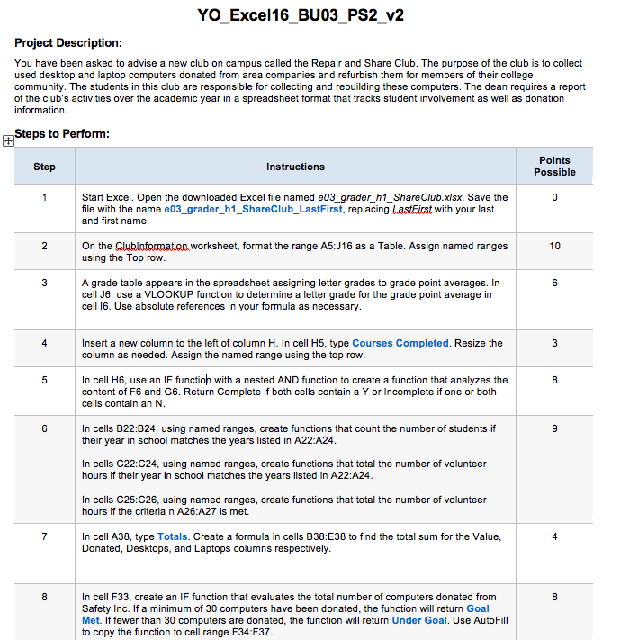
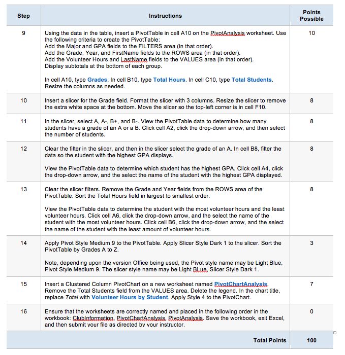
YO_Excel16_BU03_PS2_v2 Project Description: You have been asked to advise a new club on campus called the Repair and Share Club. The purpose of the club is to collect used desktop and laptop computers donated from area companies and refurbish them for members of their college community. The students in this club are responsible for collecting and rebuilding these computers. The dean requires a report of the club's activities over the academic year in a spreadsheet format that tracks student involvement as well as donation information. Steps to Perform: Step Instructions Points Possible Start Excel. Open the downloaded Excel file named e03_grader_h1_Share Club.xisx. Save the 0 file with the name e03_grader_h1_ShareClub_LastFirst, replacing LastFirst with your last and first name. 2 On the Clubloformation worksheet, format the range A5:J16 as a Table. Assign named ranges 10 using the Top row. 3 A grade table appears in the spreadsheet assigning letter grades to grade point averages. In 6 cell J6, use a VLOOKUP function to determine a letter grade for the grade point average in cell 16. Use absolute references in your formula as necessary. 4 Insert a new column to the left of column H. In cell H5, type Courses Completed. Resize the 3 column as needed. Assign the named range using the top row. 5 In cell H6, use an IF function with a nested AND function to create a function that analyzes the 8 content of F6 and G6. Return Complete if both cells contain a Y or Incomplete if one or both cells contain an N. 6 In cells B22:B24, using named ranges, create functions that count the number of students if 9 their year in school matches the years listed in A22:A24. In cells C22:C24, using named ranges, create functions that total the number of volunteer hours if their year in school matches the years listed in A22:A24. In cells C25:C26, using named ranges, create functions that total the number of volunteer hours if the criteria n A26:A27 is met 7 In cell A38, type Totals. Create a formula in cells B38:E38 to find the total sum for the Value, 4 Donated, Desktops, and Laptops columns respectively. 8 In cell F33, create an IF function that evaluates the total number of computers donated from 8 Safety Inc. If a minimum of 30 computers have been donated, the function will return Goal Met. If fewer than 30 computers are donated, the function will return Under Goal. Use AutoFill to copy the function to cell range F34:F37.Step Instructions Points Possible Using the data in the table, insert a PivotTable in cell A10 on the PivotAnalysis worksheet. Use 10 the following criteria to create the PivotTable Add the Major and GPA fields to the FILTERS area (in that order). Add the Grade, Year, and FirstName fields to the ROWS area (in that order). Add the Volunteer Hours and LastName fields to the VALUES area (in that order). Display subtotals at the bottom of each group. In cell A10, type Grades. In cell B10, type Total Hours. In cell C10, type Total Students. Resize the columns as needed. 10 Insert a slicer for the Grade field. Format the slicer with 3 columns. Resize the slicer to remove 8 the extra white space at the bottom. Move the slicer so the top-left corner is in cell F10. 11 In the slicer, select A, A-, B+, and B-. View the PivotTable data to determine how many 8 students have a grade of an A or a B. Click cell A2, click the drop-down arrow, and then select the number of students 12 Clear the filter in the slicer, and then in the slicer select the grade of an A. In cell B8, filter the 8 data so the student with the highest GPA displays View the PivotTable data to determine which student has the highest GPA. Click cell A4, click the drop-down arrow, and the select the name of the student with the highest GPA displayed. 13 Clear the slicer filters. Remove the Grade and Year fields from the ROWS area of the 8 PivotTable. Sort the Total Hours field in largest to smallest order. View the PivotTable data to determine the student with the most volunteer hours and the least volunteer hours. Click cell A6, click the drop-down arrow, and the select the name of the student with the most volunteer hours. Click cell B6, click the drop-down arrow, and the select the name of the student with the least amount of volunteer hours. 14 Apply Pivot Style Medium 9 to the PivotTable. Apply Slicer Style Dark 1 to the slicer. Sort the 3 PivotTable by Grades A to Z. Note, depending upon the version Office being used, the Pivot style name may be Light Blue, Pivot Style Medium 9. The slicer style name may be Light Blue, Slicer Style Dark 1. 15 Insert a Clustered Column PivotChart on a new worksheet named PivotChartAnalysis. 7 Remove the Total Students field from the VALUES area. Delete the legend. In the chart title, replace Total with Volunteer Hours by Student. Apply Style 4 to the PivotChart. 16 Ensure that the worksheets are correctly named and placed in the following order in the 0 workbook: Clubloformation. PixofChariAnalysis, PivotAnalysis. Save the workbook, exit Excel, and then submit your file as directed by your instructor. Total Points 100