Hi, math experts. I am recently learning from Pattern Recognition and Machine Learning, Chris Bishop. Please provide a detailed explainations briefly for the following sections.

1. Section 1.2.2 Expectations and Covariances

(Page 19 - 20)

2. Section 1.2.3 Bayesian Probabilities

(Page 21 - 24)

3. Section 1.2.4 The Gaussian distribution

(Page 24 - 27)

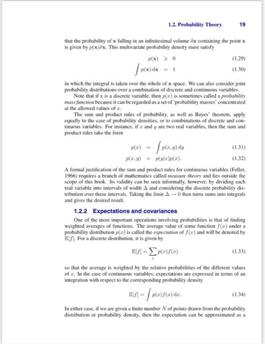
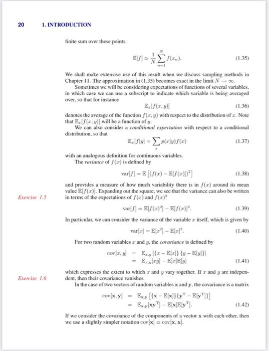
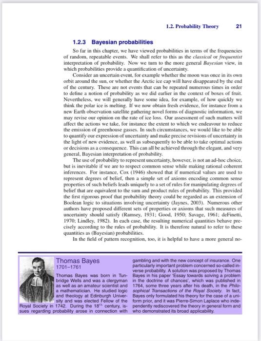
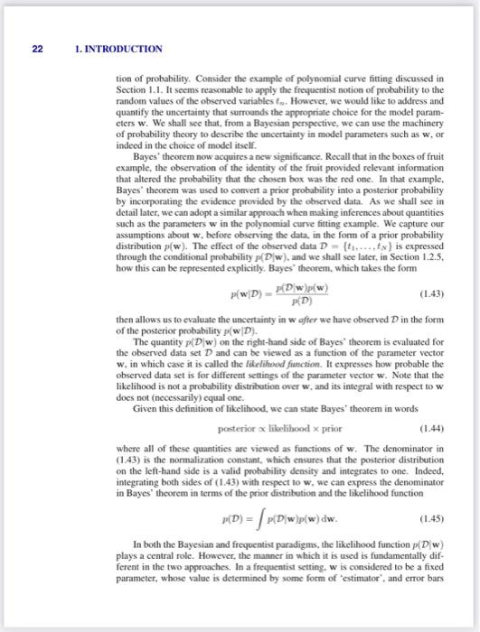
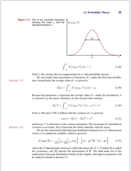
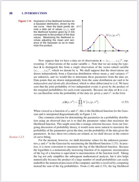
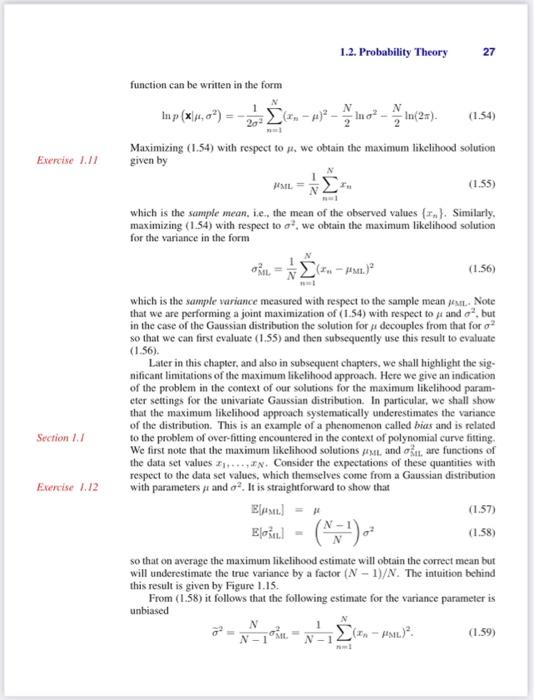
that the probability of x falling in an infinitesimal volume x containing the point x is given by p(x)x. This multivariate probability density must satisfy p(x)0p(x)dx=1 in which the integral is taken over the whole of x space. We can also consider joint probability distributions over a combination of discrete and continuous variables. Note that if x is a discrete variable, then p(x) is sometimes called a probability mass function because it can be regarded as a set of "probability masses' concentrated at the allowed values of x. The sum and product rules of probability, as well as Bayes" theorem, apply equally to the case of probability densitics, or to combinations of discrete and continuous variables. For instance, if x and y are two real variables, then the sum and product rules take the form p(x)p(x,y)=p(x,y)dy=P(yx)p(x). A formal justification of the sum and product rules for continuous variables (Feller. 1966) requires a branch of mathematics called measure theory and lies outside the scope of this book. Its validity can be seen informally, however, by dividing each real variable into intervals of width and considering the discrete probability distribution over these intervals. Taking the limit 0 then turns sums into integrals and gives the desired result. 1.2.2 Expectations and covariances One of the most important operations imvolving probabilities is that of finding weighted averages of functions. The average value of some function f(x) under a probability distribution p(x) is called the expectation of f(x) and will be denoted by E. [f]. For a discrete distribution, it is given by Ef=xg(x)f(x) so that the average is weighted by the relative probabilities of the different values of x. In the case of continuous variables, expectations are expressed in terms of an integration with respect to the corresponding probability density Bf=p(x)f(x)dx In either case, if we are given a finite number N of points drawn from the probability distribution or probability density, then the expectation can be approximated as a finite sum over these points B[f]N1n=1Nf(xn). We shall make extensive use of this result when we iscuss sampling methods in Chapter 11. The approximation in (1.35) becomes exact in the limit N. Sometimes we will be considering expectations of functions of several variables. in which case we can use a subscript to indicate which variable is being averaged over, so that for instance Exf(x,y) denotes the average of the function f(x,y) with respect to the distritution of x. Note that Ex[f(x,y)] will be a function of y. We can also consider a conditional expectation with respect to a conditional distribution, so that Zx[fy]=xp(xy)f(x) with an analogous definition for continuous variables. The variance of f(x) is defined by var[f]=E[(f(x)Z[f(x)])2] and provides a measure of how much variability there is in f(x) around its mean value E[f(x)]. Expanding out the square, we see that the variance can also be written in terms of the expectations of f(x) and f(x)2 var[f]=Ef(x)2E[f(x)]2. In particular, we can consider the variance of the variable x itself, which is given by var[x]=Ex2E[x]2 For two random variables x and y, the covariance is defined by cov[x,y]=Ex,y[{xE[x]}{yZ[y]}]=Ex,y[xy]E[x]Z[y] which expresses the extent to which x and y vary together. If x and y are independent, then their covariance vanishes. In the case of two vectors of random variables x and y, the covariance is a matrix covx,y=Ex,y[{xEx}{yEyT}] =Ex,y[xy]E[x][y]. If we consider the covariance of the components of a vector x with each other, then we use a slightly simpler notation cov[x]cov[x,x]. 1.2.3 Bayesian probabilities So far in this chapter, we have viewed probabilities in terms of the frequencies of random, repeatable events. We shall refer to this as the classical or frequentist interpretation of probability. Now we turn to the more general Baryesian view, in which probabilities provide a quantification of uncertainty. Consider an uncertain event, for example whether the moon was once in its own orbit anound the sun, or whether the Arctic ice cap will have disappeared by the end of the century. These are not events that can be repeated numerous times in order to define a notion of probability as we did earlier in the context of boxes of fruit. Nevertheless, we will generally have some idea. for example, of how quickly we think the polar ice is melting. If we now obtain fresh evidence, for instance from a new Earth observation satellite gathering novel forms of diagnostic information, we may revise our opinion on the rate of ice loss. Our assessment of such matters will affect the actions we take, for instance the extent to which we endeavour to reduce the emission of greenhouse gasses. In such circumstances, we would like to be able to quantify our expression of uncertainty and make precise revisions of uncertainty in the light of new evidence, as well as subsequently to be able to take optimal actions or decisions as a consequence. This can all be achieved through the elegant, and very general. Bayesian interpretation of probability. The use of probability to represent uncertainty, however, is not an ad-hoc choice. but is inevitable if we are to respect common sense while making rational coherent inferences. For instance, Cox(1946) showed that if numerical values are used to represent degrees of belief, then a simple set of axioms encoding common sense properties of such beliefs leads uniquely to a set of rules for manipulating degrees of belief that are equivalent to the sum and product rules of probability. This provided the first rigorous proof that probability theory could be regarded as an extension of Boolean logic to situations involving uncertainty (Jaynes, 2003). Numerous other authors have proposed different sets of properties or axioms that such measures of uncertainty should satisfy (Ramsey, 1931; Good, 1950; Savage, 1961; deFinetti, 1970: Lindley, 1982). In each case, the resulting numerical quantities behave precisely according to the rules of probability. It is therefore natural to refer to these quantities as (Bayesian) probabilities. In the field of pattern recognition, too, it is helpful to have a more general no- tion of probability. Consider the example of polynomial curve fitting discussed in Section 1.1. It seems reasonable to appily the frequentist notion of probability to the random values of the observed variables tn. However, we would like to address and quantify the uncertainty that surroands the appropriate choice for the model parameters w. We shall see that, from a Bayesian perspective, we can use the machinery of probability theory to describe the uncertainty in model parameters such as w, or indeed in the choice of model itself. Bayes' theorem now acquires a new significance. Recall that in the boxes of fruit example, the observation of the identity of the fruit provided relevant information that altered the probability that the chosen box was the red one. In that example, Bayes" theorem was used to convert a prior probability into a posterior probability by incorporating the evidence provided by the observed data. As we shall see in detail later, we can adopt a similar approach when making inferences about quantities such as the parameters w in the polynomial curve fitting example. We capture our assumptions about w, before observing the data, in the form of a prior probability distribution p(w). The effect of the observed data D={t1,,tN} is expressed through the conditional probability P(D(w), and we shall see later, in Section 1.2.5. how this can be represented explicitly. Bayes' theorem, which takes the form p(wD)=p(D)p(D;w)p(w) then allows us to evaluate the uncertainty in w offer we have observed D in the form of the posterior probability p(wD). The quantity p(Dw) on the right-hand side of Bayes' theorem is evaluated for the observed data set D and can be viewed as a function of the parameter vector w, in which case it is called the fikelihood function. It expresses how probable the observed data set is for different settings of the parameter vector w. Note that the likelihood is not a probability distribution over w, and its integral with respect to w does not (necessarily) cqual one. Given this definition of likelihood, we can state Bayes' theorem in words pasterior x likelihood prior where all of these quantities are viewed as functions of w. The denominator in (1.43) is the normalization constant, which ensures that the posterior distribution on the left-hand side is a valid probability density and integrates to one. Indeed. integrating both sides of (1.43) with respect to w, we can express the denominator in Bayes" theorem in terms of the prior distribution and the likelihood function u(D)=P(D(w)p(w)dw. In both the Bayesian and frequentist paradigms, the likelihood function p(Dw) plays a central role. However, the manner in which it is used is fundamentally different in the two approaches, In a frequentist setting, w is considered to be a fixed parameter, whose value is determined by some form of "estimator", and error bars on this estimate are obtained by considering the distribution of possible data sets D. By contrast, from the Bayesian viewpoint there is only a single data set D (namely the one that is actually observed), and the uncertainty in the parameters is expressed through a probability distribution over w. A widely used frequentist estimator is maximum likelihood, in which w is set to the value that maximizes the likelihood function p(Dw). This corresponds to choosing the value of w for which the probability of the observed data set is maximized. In the machine learning literature, the negative log of the likelihood function is called an error function. Because the negative logarithm is a monotonically decreasing function, maximizing the likelihood is equivalent to minimizing the error. One approach to determining frequentist error bars is the boofstrap (Efron, 1979; Hastie ef al., 2001), in which multiple data sets are created as follows. Suppose our original data set consists of N data points X={x1,,xN}. We can create a new data set Xn by drawing N points at random from X, with replacemeat, so that some points in X may be replicated in XU, whereas other points in X may be absent from X3. This process can be repeated L times to generate L data sets each of size N and each obtained by sampling from the original data set X. The statistical accuracy of parameter estimates can then be cvaluated by looking at the variability of predictions between the different bootstrap data sets. One advantage of the Bayesian viewpoint is that the inclusion of prior knowcdge arises naturally. Suppose, for instance, that a fair-looking coin is tossed three times and lands heads each time. A classical maximum likelihood estimate of the probability of landing heads would give 1. implying that all future torses will land heads! By contrast, a Bayesian approach with any reasonable prior will lead to a much less extreme conclusion. There has been much controversy and debate associated with the relative merits of the frequentist and Bayesian paradigms, which have not been helped by the fact that there is no unique frequentist, or even Bayesian, viewpoint. For instance, one common criticism of the Bayesian approach is that the prior distribution is often selected on the basis of mathematical convenience rather than as a reflection of any prior beliefs. Even the subjective nature of the conclusions through their dependence on the choice of prior is seen by some as a source of difficulty. Reducing the dependence on the prior is one motivation for so-called noninfomative priors. However, these lead to difficulties when comparing different models, and indeed Bayesian methods based on poor choices of prior can give poor results with high confidence. Frequentist evaluation methods offer some protection from such problems, and techniques such as cross-validation remain useful in areas such as model comparison. This book places a strong emphasis on the Bayesian viewpoint, reflecting the huge growth in the practical importance of Bayesian methods in the past few years, while also discussing useful frequentist concepts as required. Although the Bayesian framework has its origins in the 18th century, the practical application of Bayesian methods was for a long time severely limited by the difficulties in earrying through the full Bayesian procedure, particularly the need to marginalize (sum or integrate) over the whole of parameter space, which, as we shall see, is required in order to make predictions or to compare different models. The development of sampling methods, such as Markov chain Monte Carfo (discussed in Chapter 11) along with dramatic improvements in the speed and memory capacity of computers, opened the door to the practical use of Bayesian techniques in an impressive range of problem domains. Monte Carlo methods are very flexible and can be applied to a wide range of models. However, they are computationally intensive and have mainly been thed for small-scale problems. More recently, highly efficient deterministic approximation schemes such as variational Bayes and expectation propagation (discussed in Chapter 10) have been developed. These offer a complementary alternative to sampling methods and have allowed Bayesian techniques to be used in large-scale applications (Blei et al., 2003). 1.2.4 The Gaussian distribution We shall devote the whole of Chapter 2 to a study of various probability distributions and their key properties. It is convenient, however, to introduce bere one of the most important probability distributions for continuous variables, called the normal or Gaussian distribution. We shall make extensive tuse of this distribution in the remainder of this chapter and indeed throughout much of the book. For the case of a single real-valued variable x, the Gaussian distribution is defined by N(x,2)=(22)1/21exp{2a21(x)2} ance. The square root of the variance. given by , is called the standard deviation, and the reciprocal of the variance, written as =1/2. is called the precision. We shall see the motivation for these terms shortly. Figure 1.13 shows a plot of the Gaussian distribution. From the form of (1.46) we see that the Gaussian distribation satisfies N(x,2)>0. Everise 1.7 Also it is straightforward to show that the Gaussian is normalized, so that Plot of the univariate Gaussiar showing the mean j and the standard deviation o. N(x],2)dx=1. Thus (1.46) satisfies the two requirements for a valid probability density. We can readily find expectations of functions of x under the Gaussian distribution. In particular, the average value of x is given by D[x]=N(x,2)xdx=. Because the parameter repesents the average value of x under the distribution, it is referred to as the mean. Similarly, for the second order moment Fx2=N(x,2)x2dx=2+a2. From (1.49) and (1.50), it follows that the variance of x is given by var[x]=Zx2]Z(x)2=2 and hence 2 is referred to as the variance parameter. The maximum of a distribution is known as its mode. For a Gaussian, the mode coincides with the mean. We are also interested in the Gaussian distribution defined over a D-dimensional vector x of continuous variables, which is given by N(x,)=(2x)D/21{1/21exp{21(x)T1(x)} where the D-dimensional vector is called the mean, the DD matrix is called the covariance, and denotes the determinant of . We shall make use of the multivariate Gaussian distribution briefly in this chapter, although its properties will be studied in detail in Section 2.3. Illustration of the likelihood function for a Gaussian distribution, shown by the red curve. Here the biack points denote a data sot of values {x2}, and the likelihood function given by (1.53) corresponds to the product of the biue values. Maximizing the likelihood involves adjusting the mean and variance of the Gaussian 50 as to maxomize this product. Now suppose that we have a data set of observations x=(x1,,xN)T, representing N observations of the scalar variable x. Note that we are using the typeface X to distinguish this from a single observation of the vector-valued variable (x1,xD)T, which we denote by x. We shall suppose that the observations are drawn independently from a Gaussian distribution whose mean and variance 2 are unknown, and we would like to determine these parameters from the data set. Data points that are drawn independently from the same distribution are said to be independent and idemtically distribusted, which is often abbreviated to i.i.d. We have seen that the joint probability of two independent events is given by the product of the marginal probabilities for each event separately. Because our data set X is i.i.d., we can therefore write the probability of the data set, given and a2, in the form P(x,2)=x=1NN(xm,2). When viewed as a function of and 2, this is the likelihood function for the Gaussian and is interpreted diagrammatically in Figure 1.14. One common criterion for determining the parameters in a probability distribution using an observed data set is to find the parameter values that maximize the likelihood function. This might seem like a strange criterion because, from our foregoing discussion of probability theory, it would seem more natural to maximize the probability of the parameters given the data, not the probability of the data given the parameters. In fact, these two criteria are related, as we shall discuss in the context of curve fitting. For the moment, however, we shall determine values for the unknown parameters and 2 in the Gaussian by maximizing the likelihood function (1.53). In practice, it is more convenient to maximize the log of the likelihood function. Because the logarithm is a monotonically increasing function of its argument, maximization of the log of a function is equivalent to maximization of the function itself. Taking the log not only simplifies the subsequent mathematical analysis, but it also helps numerically because the product of a large number of small probabilities can easily underflow the numerical precision of the compaler, and this is resolved by computing instead the sum of the log probabilities. From (1.46) and (1.53), the log likelihood 1.2. Probability Theory 27 function can be written in the form lnp(x,2)=221n=1N(xn)22Nln22Nln(2). Maximizing ( 1.54 ) with respect to , we obtain the maximum likelihood solution given by MLL=N1n=1Nxn which is the sampte mean, i.e., the mean of the observed values {xn}. Similarly, maximizing (1.54) with respect to 2, we obain the maximum likelihood solution for the variance in the form MLL2=N1n=1N(xnML.)2 which is the sample variance measured with respect to the sample mean MLL. Note that we are performing a joint maximization of (I.54) with respect to and a2, but in the case of the Gaussian distribution the solution for decouples from that for 2 so that we can first evaluate (1.55) and then subsequently use this result to evaluate (1.56). Later in this chapter, and also in subsequent chapters, we shall highlight the significant limitations of the maximum likelihood approach. Here we give an infication of the problem in the context of our solutions for the maximum likelihood parameter settings for the univariate Gaussian distribution. In particular, we shall show that the maximum likelihood approach systematically underestimates the variance of the distribution. This is an example of a phenomenon called bias and is related to the problem of over-fitting encountered in the context of polynomial curve fitting. We first note that the maximum likelihood solutions ML and S.t,2 are functions of the data set values x1,xN. Consider the expectations of these quantities with respect to the data set values, which themselves come from a Gaussian distribution with parameters and 2. It is straightforward to show that E[MAt]=E[ML.2]=(NN1)2 so that on average the maximum likelihood estimate will obtain the correct mean but will underestimate the true variance by a factor (N1)/N. The intuition behind this result is given by Figure 1.15. From (1.58) it follows that the following estimate for the variance parameter is unbiased ~2=N1NML2=N11N=1N(xnMLL)2