Hi, This is a question on Machine learning using MATLAB. Please check the the last attachment for the task to be done.

best regards

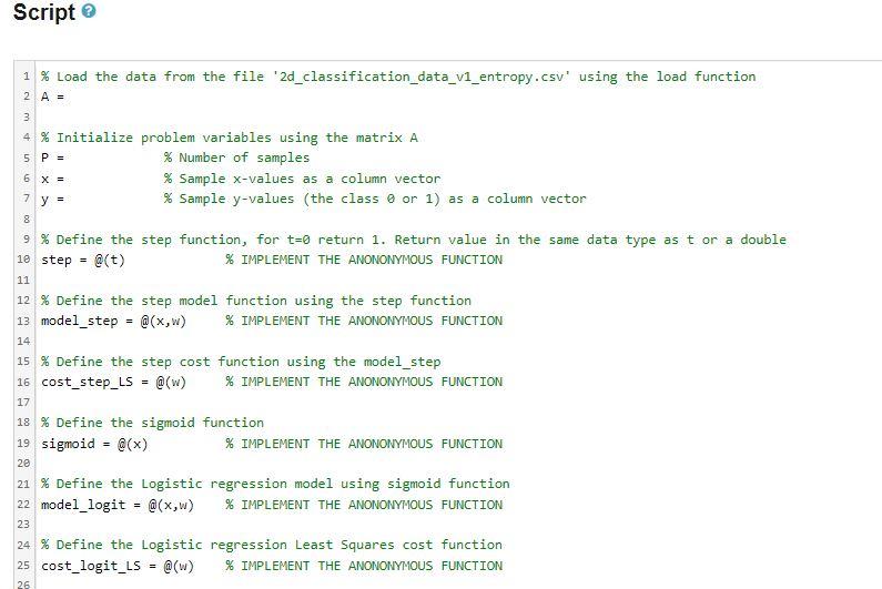
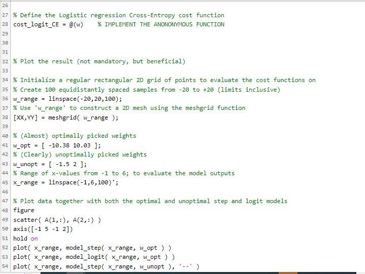
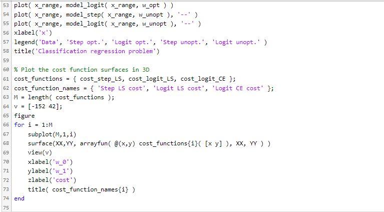
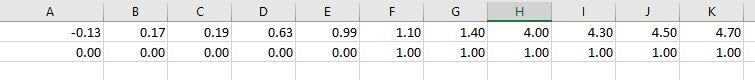
Script \% Define the Logistic regression Cross-Entropy cost function cost_logit_CE =@(w) \% IMPLEMENT THE ANONONYMOUS FUNCTION % Plot the result (not mandatory, but beneficial) \% Initialize a regular rectangular 20 grid of points to evaluate the cost functions on % Create 100 equidistantly spaced samples from 20 to +20 (limits inclusive) w_range = linspace (20,20,100); \% Use "W_range' to construct a 20 mesh using the meshgrid function [XX,YY]= meshgrid (w_range ); \% (Almost) optimally picked weights wopt=[10.3810.03]; % (Clearly) unoptimally picked weights W_unopt =[1.52]; % Range of x-values from 1 to 6 ; to evaluate the model outputs x range = linspace (1,6,100); \% Plot data together with both the optimal and unoptimal step and logit models figure scatter(A(1,:),A(2,:)) axis([1512]) hold on plot ( x_range, model_step(x_range, w_opt ) ) plot ( x_range, model_logit (x_range, w_opt)) plot (x_range, model_step( xrange, w_unopt), '-.') \begin{tabular}{r|r|l|l|l|l|l|l|l|l|l|l|l|} \hline A & B & C & D & E & F & G & H & I & J & K \\ \hline 0.0.13 & 0.17 & 0.19 & 0.63 & 0.99 & 1.10 & 1.40 & 4.00 & 4.30 & 4.50 & 4.70 \\ \hline 0.00 & 0.00 & 0.00 & 0.00 & 0.00 & 1.00 & 1.00 & 1.00 & 1.00 & 1.00 & 1.00 \\ \hline \end{tabular} Task In this problem, your task is to define the aforementioned models and cost functions in the code template by completing it according to the comments. The data to define the costs is given in the file named 2d_classification_data_1__entropy.csv. The file has been uploaded in to the Grader system and is also available on the course Moodle page for local development. The data file has 2 rows and 11 columns, where the first row corrensponds to the sample x-values, and the second row to the y-values, i.e. the class of the sample ( 0 or 1 ). So we have a one dimensional input variable, i.e. N=1, and there are P=11 samples of input-output variable pairs (xp,yp) in total. Both the step and sigmoid functions you implement must accept any size data matrix, and return the result in a same size matrix with the said function applied to each individual element, correspondingly. So, it does not suffice that the function would work just on a single evaluation point! Familiriaze yourself with e.g. on how the MATLAB sine function works on the input data. The model and cost functions that you complete should accept input vectors x and weights w that are given as individual row vectors or more generally given in the matrix form where each row corresponds to a one input vector or one set of weights, and the columns iterate the elements of that input/weight! Using matrix form input (like in Problem 2 of Assignment 3 ), they can then easily be evaluated over many points using linear algebra. The output of the models should have as many rows as there are rows in the input x, and as many columns as there are rows in w, the output at certain row and column index matching that pair of input vectors and weights. Note that another way to perform multipoint evaluation is to use the arrayfun function without the need for explicit for-loops, but the matrix product way is much more efficient. There are examples of the usage of the arrayfun in the plotting codes at the end of the code template. The model functions that you define, i.e. model_step and model_logit, should also work for any number of samples and for any dimensional input data, i.e. it can be that N>1 unlike in the data file! So do not hard code the models. The cost functions, i.e. cost_step_LS, cost_logit_LS, cost_logit_CE, are constructed based on the data from the file, and need not to work with any other data set. But the cost functions can be evaluated with any number of weight vectors (collected into the rows of the matrix w). The optional plotting code at the end of the code template visualises the data, and demonstrates the model outputs with optimally and unoptimally chosen parameters similarly to the Figures 6.5 and 6.7 of the course book (2nd ed.).It also shows the different cost function surfaces as three dimensional surface plots by evaluating the cost functions you define over a mesh grid of data points. It can only complete successfully, if your functions are well-defined. Otherwise, the plotting code may generate errors. The results should look like the two Figures below