How do I create the IF function on number 6 on instructions

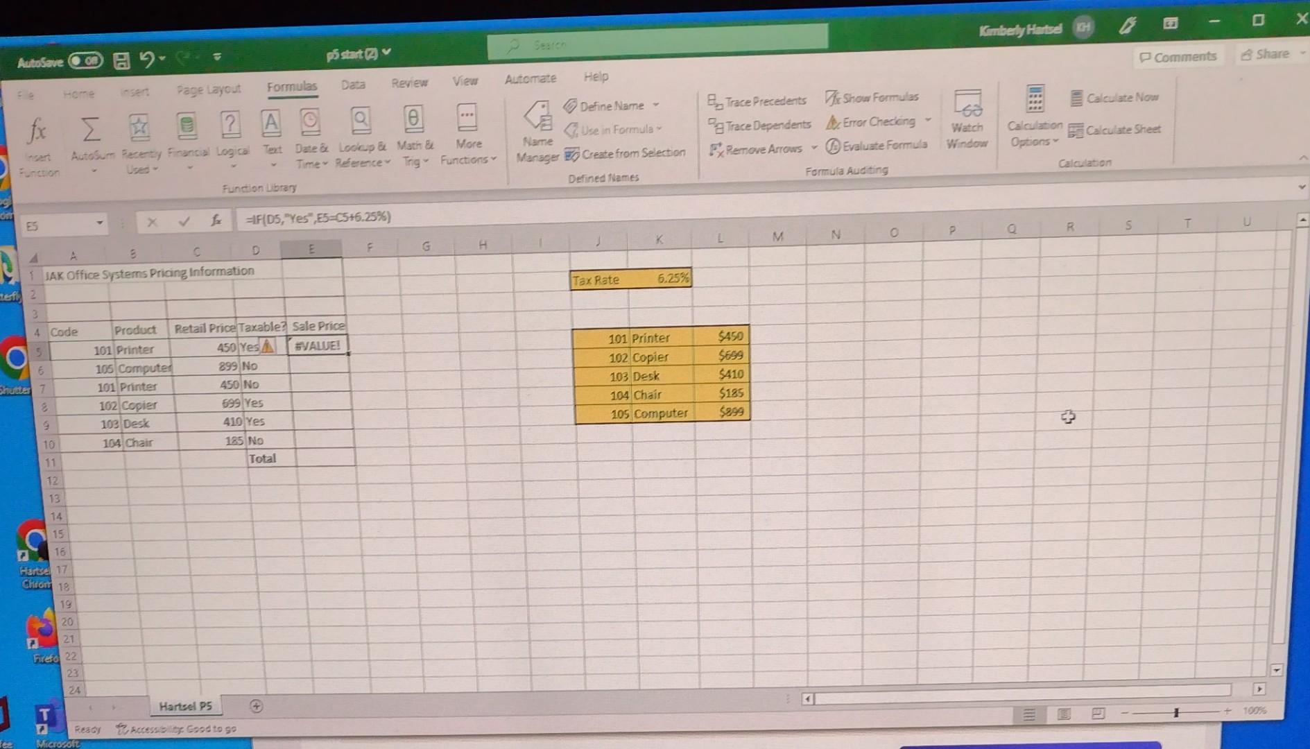
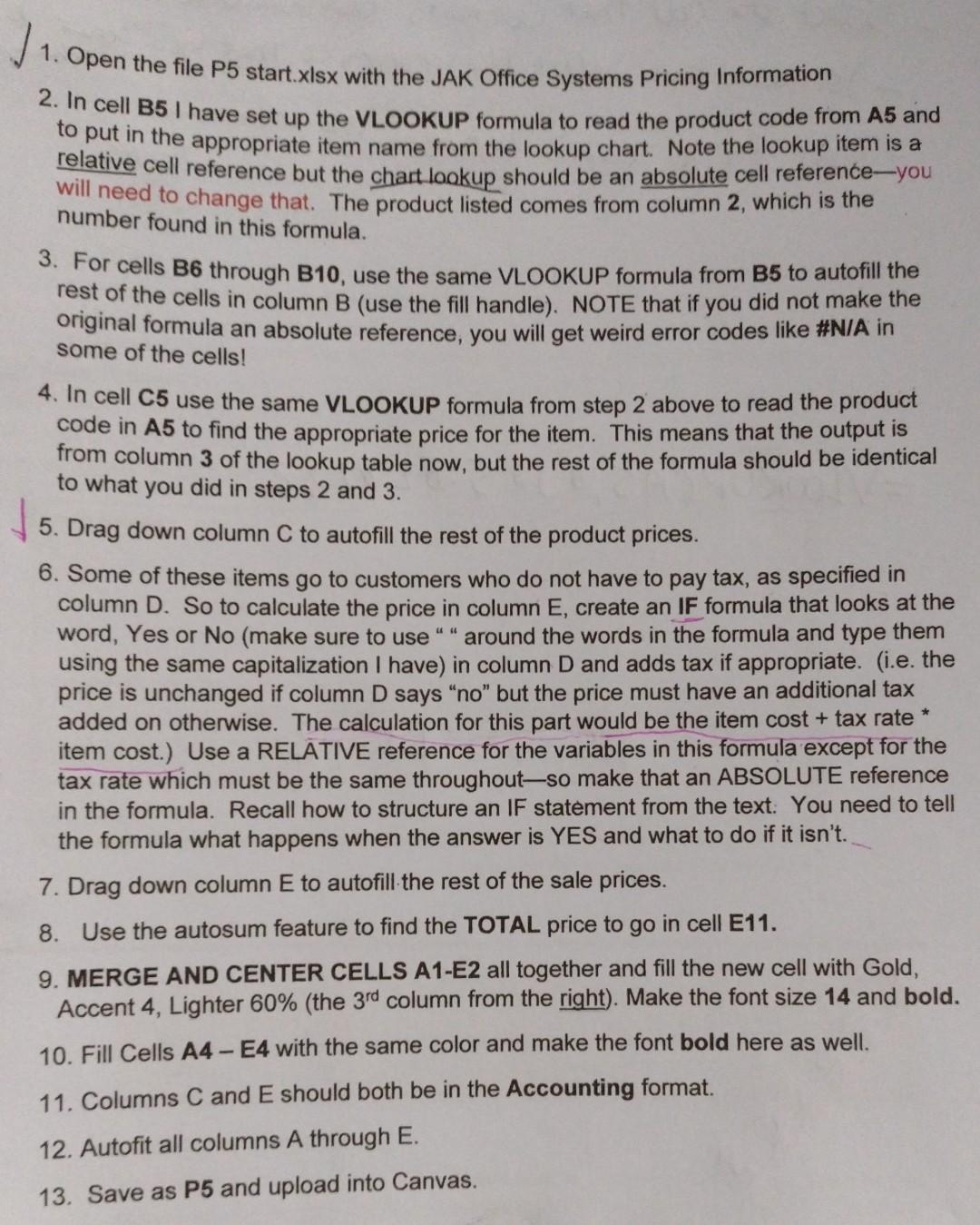
1. Open the file P5 start.xIs x with the JAK Office Systems Pricing Information 2. In cell B5 I have set up the VLOOKUP formula to read the product code from A5 and to put in the appropriate item name from the lookup chart. Note the lookup item is a relative cell reference but the chart lookup should be an absolute cell reference-you will need to change that. The product listed comes from column 2, which is the number found in this formula. 3. For cells B6 through B10, use the same VLOOKUP formula from B5 to autofill the rest of the cells in column B (use the fill handle). NOTE that if you did not make the original formula an absolute reference, you will get weird error codes like \#N/A in some of the cells! 4. In cell C5 use the same VLOOKUP formula from step 2 above to read the product code in A5 to find the appropriate price for the item. This means that the output is from column 3 of the lookup table now, but the rest of the formula should be identical to what you did in steps 2 and 3 . 5. Drag down column C to autofill the rest of the product prices. 6. Some of these items go to customers who do not have to pay tax, as specified in column D. So to calculate the price in column E, create an IF formula that looks at the word, Yes or No (make sure to use " " around the words in the formula and type them using the same capitalization I have) in column D and adds tax if appropriate. (i.e. the price is unchanged if column D says "no" but the price must have an additional tax added on otherwise. The calculation for this part would be the item cost + tax rate * item cost.) Use a RELATIVE reference for the variables in this formula except for the tax rate which must be the same throughout-so make that an ABSOLUTE reference in the formula. Recall how to structure an IF statement from the text. You need to tell the formula what happens when the answer is YES and what to do if it isn't. 7. Drag down column E to autofill the rest of the sale prices. 8. Use the autosum feature to find the TOTAL price to go in cell E11. 9. MERGE AND CENTER CELLS A1-E2 all together and fill the new cell with Gold, Accent 4 , Lighter 60% (the 3rd column from the right). Make the font size 14 and bold. 10. Fill Cells A4 - E4 with the same color and make the font bold here as well. 11. Columns C and E should both be in the Accounting format. 12. Autofit all columns A through E. 13. Save as P5 and upload into Canvas