

- How does L.L. Bean use past demand data and a specific item forecast to decide how many units of that item to stock?
- What item costs and revenues are relevant to the decision of how many units of that item to stock?
- How would you address Mark Fasolds concern that the number of items purchased usually exceeds the number forecast?
- What should L.L. Bean do to improve its forecasting process?
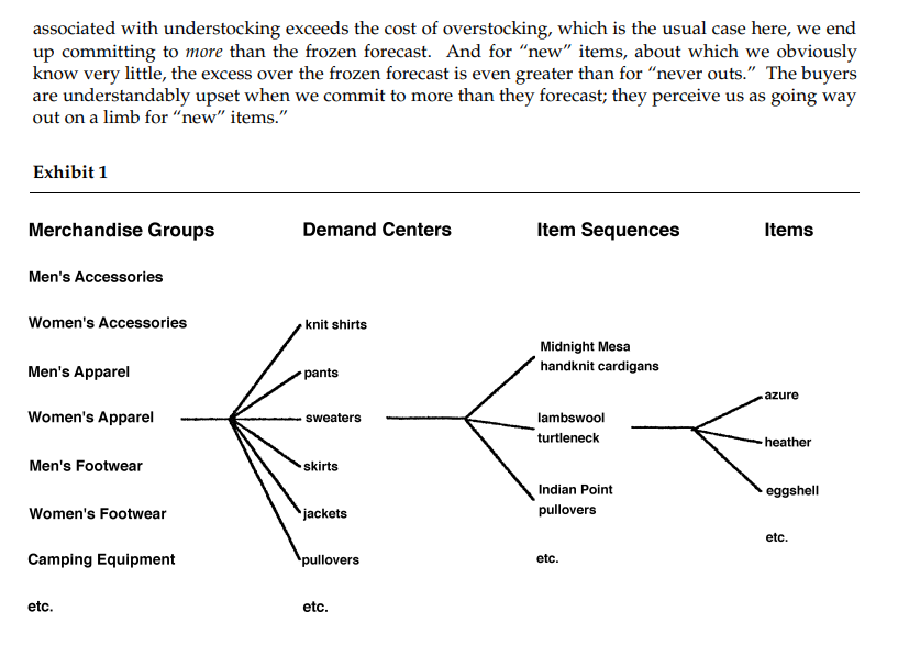
L.L. Bean's product line was classified hierarchically (see Exhibit 1). At the highest level of aggregation were Merchandise Groups: men's and women's accessories, men's and women's apparel, men's and women's footwear, camping equipment, etc. Within each Group were Demand Centers; for instance, women's apparel had as Demand Centers knit shirts, sweaters, pants, skirts, jackets and pullovers, etc. Each Demand Center was further broken down into Item Sequences; for example, women's sweaters consisted of Midnight Mesa Handknit Cardigans, Indian Point Pullovers, Lambswool Turtlenecks, and about twenty other products. Item Sequences were further broken down into individual items, distinguished primarily by color; it was at this item level that forecasts had to be issued and, ultimately, purchase commitments had to be made. 2 About 6,000 items appeared in one or another of the catalogs that were issued in the course of a year. Production Commitments The typical production lead time for most domestic orders was eight to twelve weeks. (Of course, deliveries against a commitment could be scheduled to conform to the anticipated pattern of in-season demand.) With some vendors who cooperated with L.L. Bean's "Quick Response" initiative, it was possible, after observing some early-season demand, to place a second order, which would be delivered in sufficient time to meet late-season demand. However, with many domestic and most offshore vendors, lead times were sufficiently long so that it was impractical to place a second commitment order in the course of the season. (In the remainder of this case, then, discussion will be limited to these "one-shot" commitments.) The commitments were generally not equal in size to the forecasts, but were determined in two steps as follows: First, historical forecast errors (expressed as "A/F ratios" the ratio of actual demand to forecast demand) were computed for each item in the previous year, and the frequency distribution of these errors was compiled across items. 3 The frequency distribution of past forecast errors was then used as a probability distribution for the as yet unrealized future forecast errors. For example, if 50% of the forecast errors for "new" items in the past year had been between 0.7 and 1.6, then it would be assumed that with probability 0.5, the forecast error for any "new" item in the current year also would fall between 0.7 and 1.6. So in such a case, if the frozen forecast for a particular item were 1,000 units, it was then assumed that with probability 0.5 , actual demand for that item would end up being between 700 and 1,600 units. Next, each item's commitment quantity was determined by balancing the individual item's contribution margin if demanded against its liquidation cost (or value) if not demanded. Suppose, for example, that an item cost Bean $15, would regularly sell for $30, and could be sold at liquidation for $10. The gain for selling a marginal unit would be $3015=$15; the loss for failing to sell the marginal unit would be the cost less the liquidation value, i.e. $1510=$5. Accordingly, the optimal order size should be the 0.75 fractile of the item's probability distribution of demand. Suppose the 0.75 fractile of the distribution of forecast errors was 1.3, and the frozen forecast for that item was for 1,000 units. Then the 0.75 fractile of the demand distribution would be 1,0001.3=1,300, and Bean would make a commitment for 1,300 units. Rol Fessenden expressed concern that the methodology treated the errors associated with all "never out" items as equally representative of the forecast errors that might be anticipated for the forecast demand of any "never out" item (and similarly for "new" items). "You'd think that the error distribution for some of our buyers might be tighter than for other buyers, or that the distribution for women's sweaters might have more dispersion than the distribution for men's footwear, but we can't find any real differences. Also, I'm not entirely convinced that we go about estimating contribution margin and liquidation cost correctly." Mark Fasold was worried about the wide dispersion in forecast errors, both for "never outs" and "new" items. He was also concerned about the implications of the methodology: "If the cost associated with understocking exceeds the cost of overstocking, which is the usual case here, we end up committing to more than the frozen forecast. And for "new" items, about which we obviously know very little, the excess over the frozen forecast is even greater than for "never outs." The buyers are understandably upset when we commit to more than they forecast; they perceive us as going way out on a limb for "new" items

