 HW_1_Sample _Code
HW1_Sample_Code_plot
dvd_fun_input.m
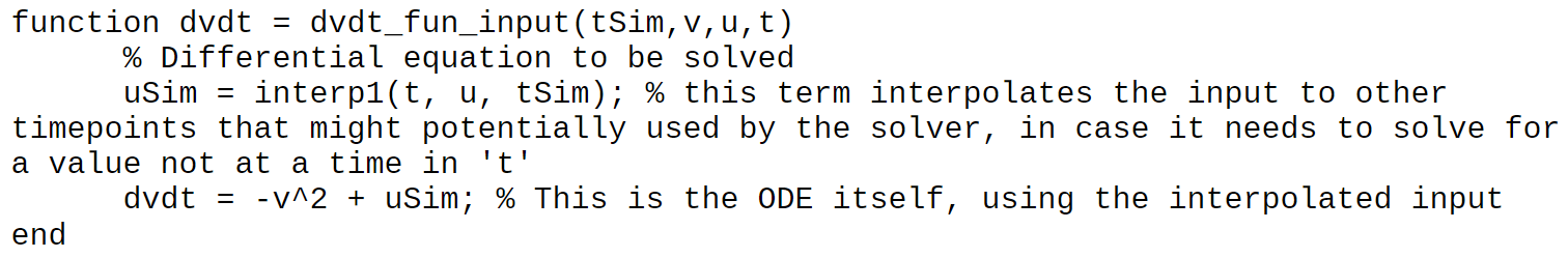
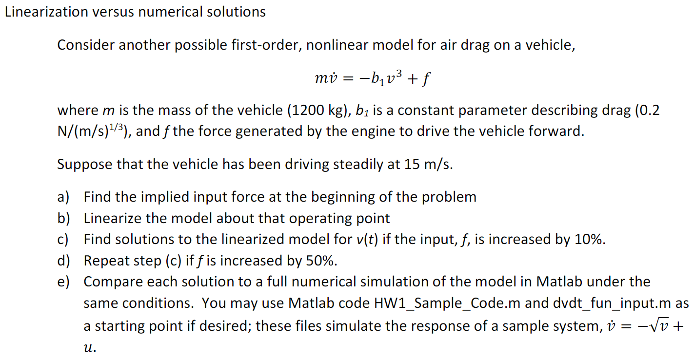
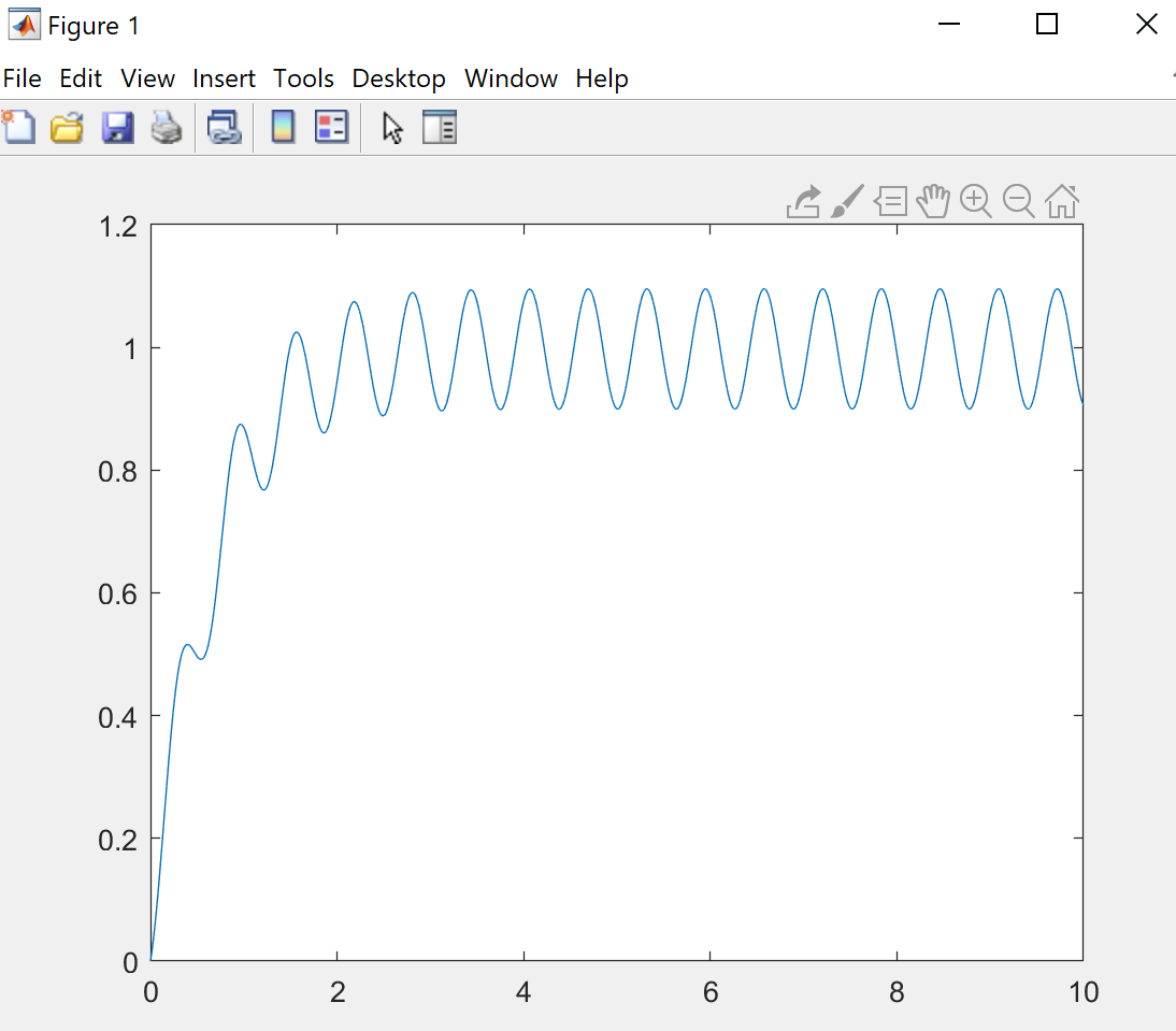
Linearization versus numerical solutions Consider another possible first-order, nonlinear model for air drag on a vehicle, m = -b1v3 +f where m is the mass of the vehicle (1200 kg), b is a constant parameter describing drag (0.2 N/(m/s)1/3), and f the force generated by the engine to drive the vehicle forward. Suppose that the vehicle has been driving steadily at 15 m/s. a) Find the implied input force at the beginning of the problem b) Linearize the model about that operating point c) Find solutions to the linearized model for v(t) if the input, f, is increased by 10%. d) Repeat step (c) if f is increased by 50%. e) Compare each solution to a full numerical simulation of the model in Matlab under the same conditions. You may use Matlab code HW1_Sample_Code.m and dvdt_fun_input.m as a starting point if desired; these files simulate the response of a sample system, U = -V0 + . % Sample code for a Matlab numerical ODE solution with time dependent % input % ODE solution practice VO = 0; % Initial speed Tstop = 2; % End of simulation time (s) t = 0:0.01:10; u = 1+sin(10*t); % Sample ODE solver for a Matlab ODE with time varying input % syntax is sort of complex: % ode 23 is the solution function % the @(t Sim, v) tells the solver to solve for variable y at timepoints tSim % dvdt_fun_input is a Matlab function defining the ODE, which has its own % set of variable: tSim, a set of solution times the solver may use; v, the % variable in the ODE; u, the input to the ODE; and t, the timepoints for % which the input is recorded. % Finally, the solver also needs the times at which to solve, which we use % 't' for again, for convenience, and an initial condition, 'vo'. [t, v] = ode23(@(tSim, v) dvdt_fun_input(tSim, v, u, t), t, vo); plot(t, v) % Your solution found by hand can be plotted with your adjusted model using % 'hold on'. % Note: depending on the version of Matlab you are using, you may need to % place your function here, at the bottom of the file, rather than in a % separate file. - O X Figure 1 File Edit View Insert Tools Desktop Window Help a my Q QW MW OF function dvdt = dvdt_fun_input(tSim, v, u,t) % Differential equation to be solved usim = interp1(t, u, tsim); % this term interpolates the input to other timepoints that might potentially used by the solver, in case it needs to solve for a value not at a time in 't' dvdt = -V^2 + uSim; % This is the one itself, using the interpolated input end Linearization versus numerical solutions Consider another possible first-order, nonlinear model for air drag on a vehicle, m = -b1v3 +f where m is the mass of the vehicle (1200 kg), b is a constant parameter describing drag (0.2 N/(m/s)1/3), and f the force generated by the engine to drive the vehicle forward. Suppose that the vehicle has been driving steadily at 15 m/s. a) Find the implied input force at the beginning of the problem b) Linearize the model about that operating point c) Find solutions to the linearized model for v(t) if the input, f, is increased by 10%. d) Repeat step (c) if f is increased by 50%. e) Compare each solution to a full numerical simulation of the model in Matlab under the same conditions. You may use Matlab code HW1_Sample_Code.m and dvdt_fun_input.m as a starting point if desired; these files simulate the response of a sample system, U = -V0 + . % Sample code for a Matlab numerical ODE solution with time dependent % input % ODE solution practice VO = 0; % Initial speed Tstop = 2; % End of simulation time (s) t = 0:0.01:10; u = 1+sin(10*t); % Sample ODE solver for a Matlab ODE with time varying input % syntax is sort of complex: % ode 23 is the solution function % the @(t Sim, v) tells the solver to solve for variable y at timepoints tSim % dvdt_fun_input is a Matlab function defining the ODE, which has its own % set of variable: tSim, a set of solution times the solver may use; v, the % variable in the ODE; u, the input to the ODE; and t, the timepoints for % which the input is recorded. % Finally, the solver also needs the times at which to solve, which we use % 't' for again, for convenience, and an initial condition, 'vo'. [t, v] = ode23(@(tSim, v) dvdt_fun_input(tSim, v, u, t), t, vo); plot(t, v) % Your solution found by hand can be plotted with your adjusted model using % 'hold on'. % Note: depending on the version of Matlab you are using, you may need to % place your function here, at the bottom of the file, rather than in a % separate file. - O X Figure 1 File Edit View Insert Tools Desktop Window Help a my Q QW MW OF function dvdt = dvdt_fun_input(tSim, v, u,t) % Differential equation to be solved usim = interp1(t, u, tsim); % this term interpolates the input to other timepoints that might potentially used by the solver, in case it needs to solve for a value not at a time in 't' dvdt = -V^2 + uSim; % This is the one itself, using the interpolated input end