I am confused as too how i go forward with the Gauss-Markov Process section of this problem?
i am confused on how to go forward with the Gauss-Markov process section of this problem
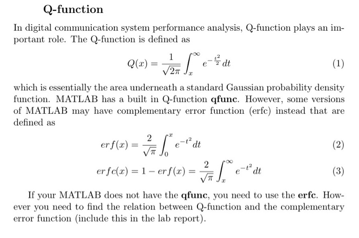
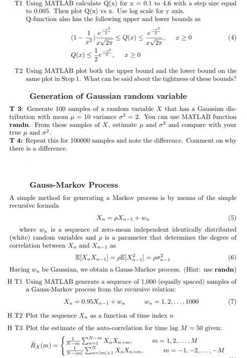
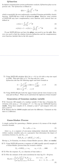
Q-function la digital.comcon system per feste plays an im portant role. The Q-functions de (1) which is entially the area understand wipeobability desity function. MATLAB aut in Q-function. How of MATLAB have complementary facto) instead that are defels If your MATLAB does not how the one you to the exfe. How ever you wed to find the relation between Q-faxed the complety error function (include this in the lab report TI Using MATLAB ete) for 16 with a step to 0.005 The plot Qx) xwe Q-function sols the following pera "NESS S. 220 To Using MATLAB plot both the bound the band on the same plot in Step 1. What can be the othebed? Generation of Gaussian random variable T3 Gate 100 ples of a random variable data Geldi tribution with many - 10 vare - 2 You MATLAB function rando. From the samples of Xestimate compare with your treando T 4: Repeat this for 100.000 samples and the Comment on why the is a difference Gauss-Markov Process A simple method for generating a Martorpeces is by ses of the simple where w, is a ce of indepedra idrically distributed (white) random variables and is ter that determines the degree of correlation between XX. Haring, be used, we obtain a Go-Maroc (Hitrandn) HTI Using MATLAB of emples of G-Meelow process from the received 12 HT2 Plot there X, as a function of the HT3 Plot the estimate of the worlati fog M 50g X.X... (8) Q-function In digital communication system performance analysis, Q-function plays an im- portant role. The Q-function is defined as 1 Q(x) = (1) 27 which is essentially the area underneath a standard Gaussian probability density function. MATLAB has a built in Q-function qfunc. However, some versions of MATLAB may have complementary error function (erfc) instead that are defined as 2 er f(x) e-t dt V (2) 2 er fc(x) = 1 - erf(x) = (3) V/ If your MATLAB does not have the qfunc, you need to use the erfc. How- ever you need to find the relation between Q-function and the complementary error function (include this in the lab report). Ti Using MATLAB calculate Q(x) for x = 0.1 to 4.6 with a step size equal to 0.005. Then plot Q(x) vs x. Use log scale for y axis. Q-function also has the following upper and lower bounds as le* *** (1 SQ() IV 2 r> 0 IV 2 Q(r)se, 120 T2 Using MATLAB plot both the upper bound and the lower bound on the same plot in Step 1. What can be said about the tightness of these bounds? Generation of Gaussian random variable T 3: Generate 100 samples of a random variable X that has a Gaussian dis- tribution with mean u = 10 variance o2 = 2. You can use MATLAB function randn. From these samples of X, estimate and oand compare with your true and T 4: Repeat this for 100000 samples and note the difference. Comment on why there is a difference. Gauss-Markov Process A simple method for generating a Markov process is by means of the simple recursive formula Xn=pXn-1 + win (5) where wn is a sequence of zero-mean independent identically distributed (white) random variables and p is a parameter that determines the degree of correlation between X, and Xn-1 as E[X,Xn-1] = p[X3-1] = poa-1 (6) Having W, be Gaussian, we obtain a Gauss-Markov process. (Hint: use randn) H Ti Using MATLAB generate a sequence of 1,000 (equally spaced) samples of a Gauss-Markov process from the recursive relation: X, = 0.95X-1+w w = 1,2,..., 1000 (7) H T2 Plot the sequence X, as a function of time index n HT3 Plot the estimate of the auto-correlation for time lag M = 50 given: m=1,2,....M x (m) = m = -1, -2, ...,-M N-m=1 N =m+1 SN-" X,Xn+m X.Xn+ N-m Q-function la digital.comcon system per feste plays an im portant role. The Q-functions de (1) which is entially the area understand wipeobability desity function. MATLAB aut in Q-function. How of MATLAB have complementary facto) instead that are defels If your MATLAB does not how the one you to the exfe. How ever you wed to find the relation between Q-faxed the complety error function (include this in the lab report TI Using MATLAB ete) for 16 with a step to 0.005 The plot Qx) xwe Q-function sols the following pera "NESS S. 220 To Using MATLAB plot both the bound the band on the same plot in Step 1. What can be the othebed? Generation of Gaussian random variable T3 Gate 100 ples of a random variable data Geldi tribution with many - 10 vare - 2 You MATLAB function rando. From the samples of Xestimate compare with your treando T 4: Repeat this for 100.000 samples and the Comment on why the is a difference Gauss-Markov Process A simple method for generating a Martorpeces is by ses of the simple where w, is a ce of indepedra idrically distributed (white) random variables and is ter that determines the degree of correlation between XX. Haring, be used, we obtain a Go-Maroc (Hitrandn) HTI Using MATLAB of emples of G-Meelow process from the received 12 HT2 Plot there X, as a function of the HT3 Plot the estimate of the worlati fog M 50g X.X... (8) Q-function In digital communication system performance analysis, Q-function plays an im- portant role. The Q-function is defined as 1 Q(x) = (1) 27 which is essentially the area underneath a standard Gaussian probability density function. MATLAB has a built in Q-function qfunc. However, some versions of MATLAB may have complementary error function (erfc) instead that are defined as 2 er f(x) e-t dt V (2) 2 er fc(x) = 1 - erf(x) = (3) V/ If your MATLAB does not have the qfunc, you need to use the erfc. How- ever you need to find the relation between Q-function and the complementary error function (include this in the lab report). Ti Using MATLAB calculate Q(x) for x = 0.1 to 4.6 with a step size equal to 0.005. Then plot Q(x) vs x. Use log scale for y axis. Q-function also has the following upper and lower bounds as le* *** (1 SQ() IV 2 r> 0 IV 2 Q(r)se, 120 T2 Using MATLAB plot both the upper bound and the lower bound on the same plot in Step 1. What can be said about the tightness of these bounds? Generation of Gaussian random variable T 3: Generate 100 samples of a random variable X that has a Gaussian dis- tribution with mean u = 10 variance o2 = 2. You can use MATLAB function randn. From these samples of X, estimate and oand compare with your true and T 4: Repeat this for 100000 samples and note the difference. Comment on why there is a difference. Gauss-Markov Process A simple method for generating a Markov process is by means of the simple recursive formula Xn=pXn-1 + win (5) where wn is a sequence of zero-mean independent identically distributed (white) random variables and p is a parameter that determines the degree of correlation between X, and Xn-1 as E[X,Xn-1] = p[X3-1] = poa-1 (6) Having W, be Gaussian, we obtain a Gauss-Markov process. (Hint: use randn) H Ti Using MATLAB generate a sequence of 1,000 (equally spaced) samples of a Gauss-Markov process from the recursive relation: X, = 0.95X-1+w w = 1,2,..., 1000 (7) H T2 Plot the sequence X, as a function of time index n HT3 Plot the estimate of the auto-correlation for time lag M = 50 given: m=1,2,....M x (m) = m = -1, -2, ...,-M N-m=1 N =m+1 SN-" X,Xn+m X.Xn+ N-m