I have been attempting this couple of questions for multiple hours now, and would extremely appreciate the help. Thank you!
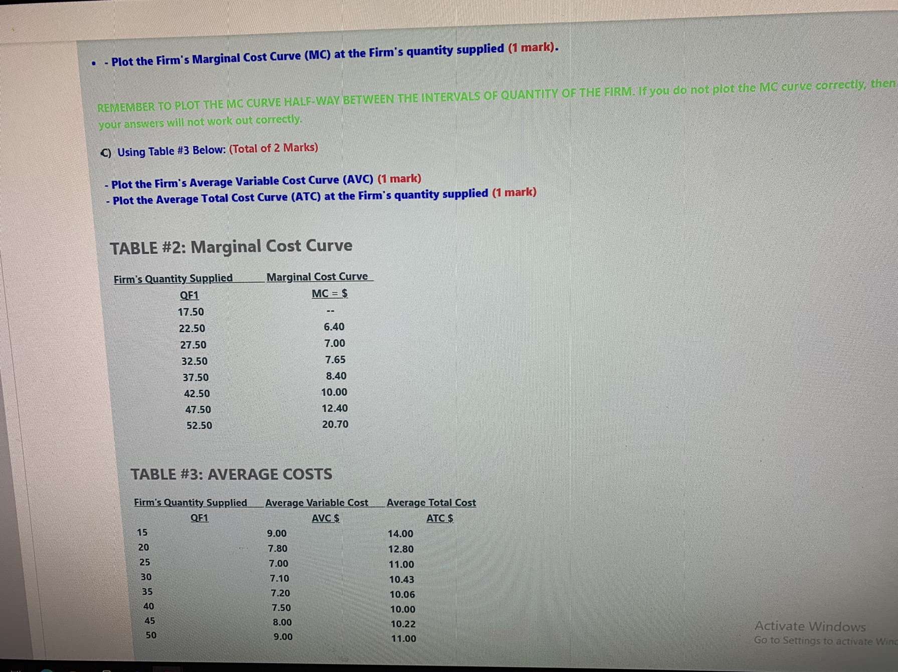
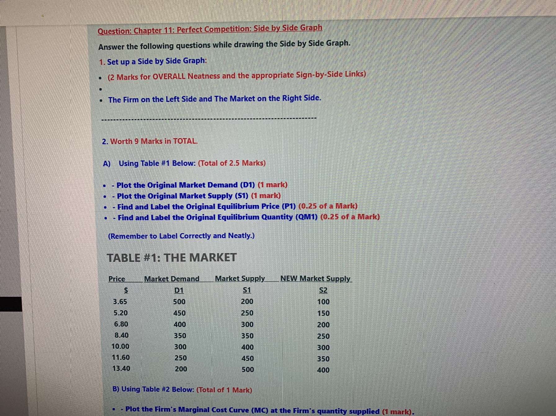
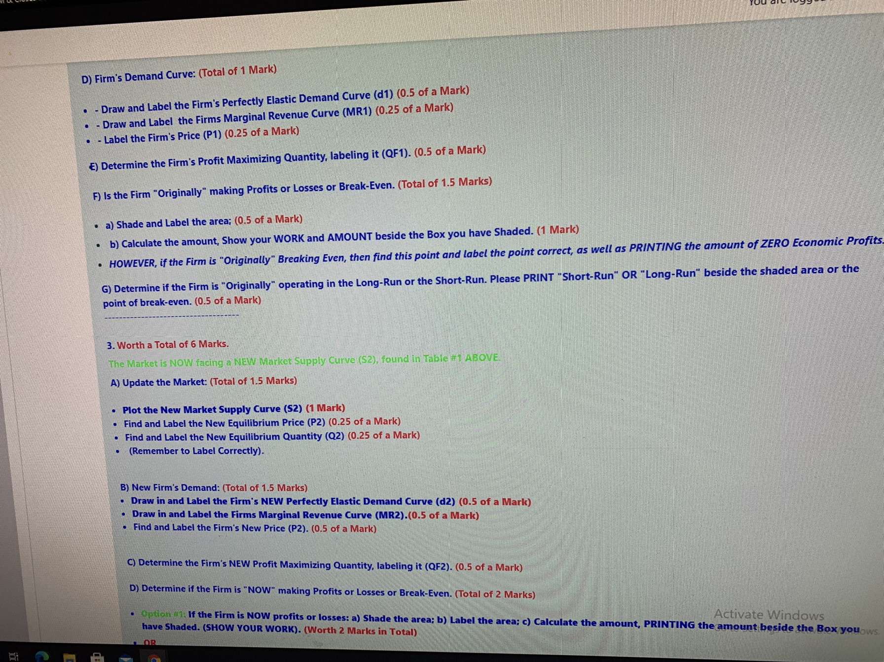
. - Plot the Firm's Marginal Cost Curve (MC) at the Firm's quantity supplied (1 mark). REMEMBER TO PLOT THE MC CURVE HALFWAY BETWEEN THE INTERVALS OF QUANTITY OF THE FIRM. If you do not plot the MC curve correctly, then your answers will not work out correctly. C) Using Table #3 Below: (Total of 2 Marks) Plot the Firm's Average Variable Cost Curve (AVC) (1 mark) Plot the Average Total Cost Curve (ATC) at the Firm's quantity supplied (1 mark) TABLE #2: Marginal Cost Curve Firm's Quantity Supplied Marginal Cost Curve OF1 MC = $. 17.50 22.50 6.40 27.50 7.00 32.50 7.65 37.50 8.40 42.50 10.00 47.50 12.40 52.50 20.70 TABLE #3: AVERAGE COSTS Firm's Quantity Supplied Average Variable Cost Average Total Cost OF1 AVC $ ATC $ 15 9.00 14.00 7.80 12.80 7.00 30 11.00 7.10 10.43 7.20 10.06 7.50 10.00 8.00 50 10.22 9.00 11.00 Activate Windows Go to Settings to activate WindQuestion: Chapter 11: Perfect Competition: Side by Side Graph Answer the following questions while drawing the Side by Side Graph. 1. Set up a Side by Side Graph: . (2 Marks for OVERALL Neatness and the appropriate Sign-by-Side Links) The Firm on the Left Side and The Market on the Right Side. 2. Worth 9 Marks in TOTAL. A) Using Table #1 Below: (Total of 2.5 Marks) - Plot the Original Market Demand (D1) (1 mark) - Plot the Original Market Supply ($1) (1 mark) - Find and Label the Original Equilibrium Price (P1) (0.25 of a Mark) . - Find and Label the Original Equilibrium Quantity (QM1) (0.25 of a Mark) (Remember to Label Correctly and Neatly.) TABLE #1: THE MARKET Price Market Demand Market Supply NEW Market Supply_ $. D1 $1 $2 3.65 500 200 100 5.20 450 250 150 6.80 400 300 200 8.40 350 350 250 10.00 300 400 300 11.60 250 450 350 13.40 200 500 400 B) Using Table #2 Below: (Total of 1 Mark) . - Plot the Firm's Marginal Cost Curve (MC) at the Firm's quantity supplied (1 mark).D) Firm's Demand Curve: (Total of 1 Mark) - Draw and Label the Firm's Perfectly Elastic Demand Curve (d1) (0.5 of a Mark) - Draw and Label the Firms Marginal Revenue Curve (MR1) (0.25 of a Mark) - Label the Firm's Price (P1) (0.25 of a Mark) E) Determine the Firm's Profit Maximizing Quantity, labeling it (QF1). (0.5 of a Mark) F) Is the Firm "Originally" making Profits or Losses or Break-Even. (Total of 1.5 Marks) a) Shade and Label the area; (0.5 of a Mark) b) Calculate the amount, Show your WORK and AMOUNT beside the Box you have Shaded. (1 Mark) HOWEVER, if the Firm is "Originally" Breaking Even, then find this point and label the point correct, as well as PRINTING the amount of ZERO Economic Profits G) Determine if the Firm is "Originally" operating in the Long-Run or the Short-Run. Please PRINT "Short-Run" OR "Long-Run" beside the shaded area or the point of break-even. (0.5 of a Mark) 3. Worth a Total of 6 Marks. The Market is NOW facing a NEW Market Supply Curve (S2), found in Table #1 ABOVE! A) Update the Market: (Total of 1.5 Marks) . Plot the New Market Supply Curve ($2) (1 Mark) Find and Label the New Equilibrium Price (P2) (0.25 of a Mark) . Find and Label the New Equilibrium Quantity (Q2) (0.25 of a Mark) (Remember to Label Correctly). 3) New Firm's Demand: (Total of 1.5 Marks) Draw in and Label the Firm's NEW Perfectly Elastic Demand Curve (d2) (0.5 of a Mark Draw in and Label the Firms Marginal Revenue Curve (MR2).(0.5 of a Mark) Find and Label the Firm's New Price (P2). (0.5 of a Mark) C) Determine the Firm's NEW Profit Maximizing Quantity, labeling it (QF2). (0.5 of a Mark) D) Determine if the Firm is "NOW" making Profits or Losses or Break-Even. (Total of 2 Marks) .Option #j. If the Firm is NOW profits or losses: a) Shade the area; b) Label the area; c) Calculate the amount, PRINTING the amount beside the Box youws. Activate Windows have Shaded. (SHOW YOUR WORK). (Worth 2 Marks in Total)


