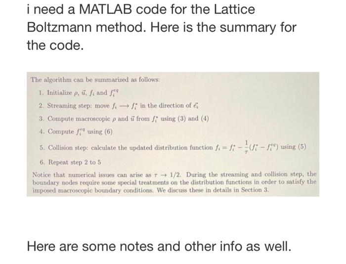
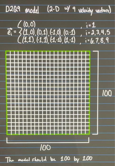
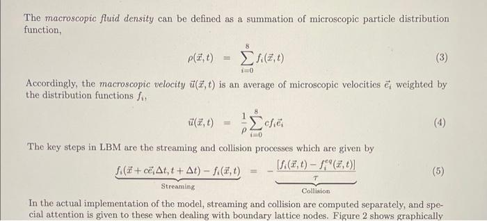
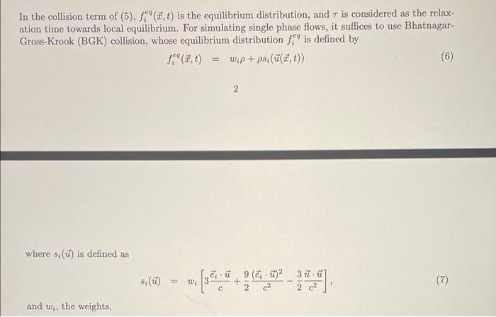
i need a MATLAB code for the Lattice Boltzmann method. Here is the summary for the code. The algorithm can be summarized as follows: 1. Initialize , . Ji and 2. Streaming step: move it fr in the direction of el 3. Compute macroscopic p and u from S: using (3) and (4) P 4. Compute ff using (6) 5. Colision steps, calculate the updated distribution function f = f* - EU: -15") using (5) 6. Repeat step 2 to 5 Notice that numerical issues can arise as T 1/2. During the streaming and collision step, the boundary nodes require some special treatments on the distribution functions in order to satisfy the imposed macroscopic boundary conditions. We discuss these in details in Section 3. Here are some notes and other info as well. . D2Q9 model (2-1 w/ a velocity vectors) ( (0,0) i=1 = 3(1,0),(0,1),(-1,0),(0-1) i= 2, 3,4,5 ((1.1), (-1,1), (1,-1), (1,-1) 7=6,7,8,9 100 100 The model should be 100 by 100 The macroscopic fluid density can be defined as a summation of microscopic particle distribution function, , 1) 10 pat) , (3) Accordingly, the macroscopic velocity (,tis an average of microscopic velocities weighted by the distribution functions for t(, t) I Cefie 10 5 The key steps in LBM are the streaming and collision processes which are given by Sc(+ c, At,t + At) - f. (8,0) [S. (,1) - L" (3,0)] (5) Streaming Collision In the actual implementation of the model, streaming and collision are computed separately, and spe- cial attention is given to these when dealing with boundary lattice nodes. Figure 2 shows graphically In the collision term of (5), ", t) is the equilibrium distribution, and is considered as the relax- ation time towards local equilibrium. For simulating single phase flows, it suffices to use Bhatnagar- Gross-Krook (BGK) collision, whose equilibrium distribution S." is defined by wip+ps (li,t)) (6) 2 where s() is defined as 8:() = w 9 (&)2 3 + 2 c2 2 c2 (7) and w., the weights