i need al the work and lab simulations and pre labs and calculations. LAB SIMULATIONS MUST BE ON PROTEUS ISIS

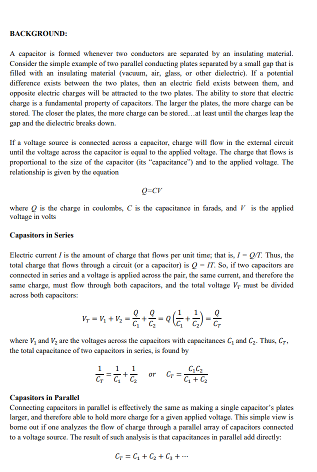
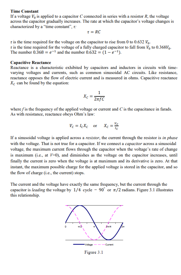
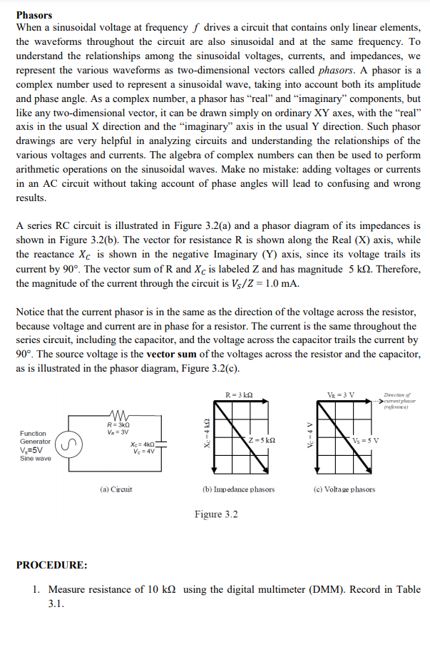
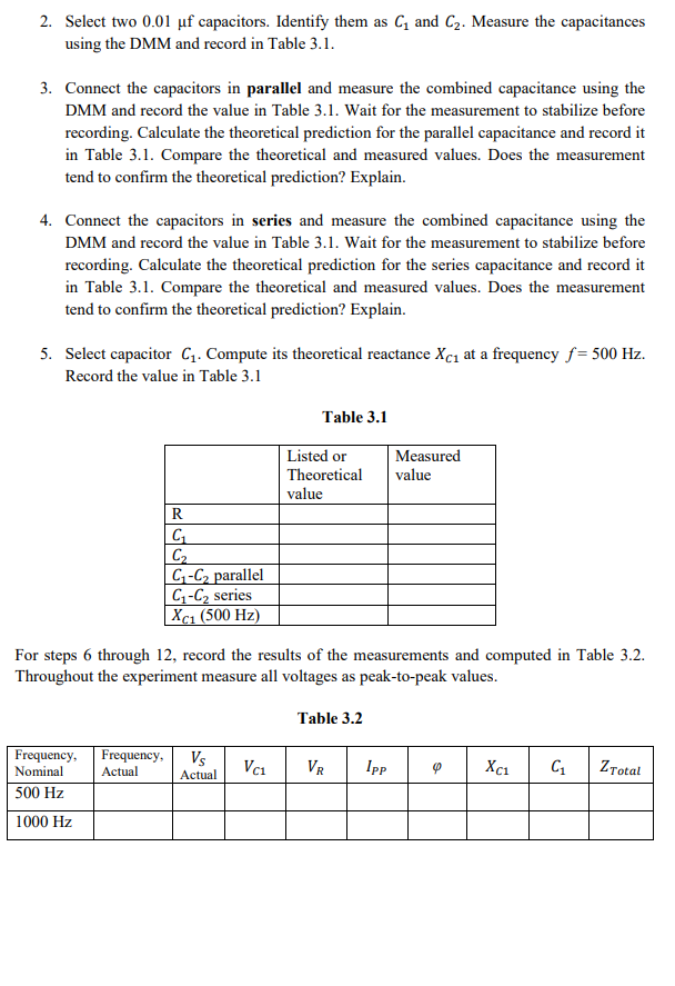
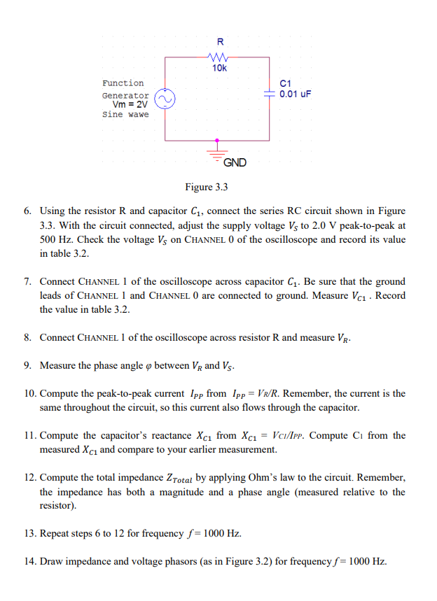
INTRODUCTION: Linear circuit elements resistors, capacitors, and inductors are the backbone of electrical and electronic circuits. These three types of elements respond to electrical voltages in different ways, variously consuming, storing, or supplying electrical energy. Understanding these behaviors and learning to calculate the result of combining elements is critical for designing and working with electric circuits. While a resistor consumes electrical energy, converting it to heat, capacitors and inductors vary their responses according to the frequency of the voltage or current applied to them. This laboratory will explore those responses for series-connected capacitors. EDUCATIONAL OBJECTIVE: (1) Learn to measure capacitive reactance and phase angles between voltages. (2) Learn to draw impedance and voltage phasor diagrams for resistors and capacitors in series. (3) Understand how impedance and voltage phasors add (i.e., like vectors). (4) Learn to simulate AC series circuit. EXPERIMENTAL OBJECTIVE: (1) Confirm how capacitances add when two capacitors are connected in parallel; in series. (2) Determine the reactance of a capacitor in a series RC circuit by measuring voltages. (3) Draw impedance and voltage phasor diagrams for a series RC circuit. (4) Explain the effect of frequency on the impedance and voltage phasors for a series RC circuit. PRE-LAB: (1) Read and study the Background section of this Laboratory. (1) In your lab notebook sketch the circuit diagram to be used in the procedure and prepare Tables 3.1 and 3.2 to record data. Sketch the impedance and voltage phasors diagrams (as in Figure 3.2) you would get at 500 Hz for the circuit in Figure 3.3. Make a table of the magnitudes and phase angles. You will use this to check that your experimental setup is correct. EQUIPMENT NEEDED: Function Generator Digital Multimeter (DMM) Oscilloscope 1x 10 K resistor 2 x 0.01uF capacitors . BACKGROUND: A capacitor is formed whenever two conductors are separated by an insulating material. Consider the simple example of two parallel conducting plates separated by a small gap that is filled with an insulating material (vacuum, air, glass, or other dielectric). If a potential difference exists between the two plates, then an electric field exists between them, and opposite electric charges will be attracted to the two plates. The ability to store that electric charge is a fundamental property of capacitors. The larger the plates, the more charge can be stored. The closer the plates, the more charge can be stored...at least until the charges leap the gap and the dielectric breaks down. If a voltage source is connected across a capacitor, charge will flow in the external circuit until the voltage across the capacitor is equal to the applied voltage. The charge that flows is proportional to the size of the capacitor (its capacitance") and to the applied voltage. The relationship is given by the equation Q=CV where is the charge in coulombs, C is the capacitance in farads, and V is the applied voltage in volts Capasitors in Series Electric current I is the amount of charge that flows per unit time; that is, I = Q/T. Thus, the total charge that flows through a circuit (or a capacitor) is Q = IT. So, if two capacitors are connected in series and a voltage is applied across the pair, the same current, and therefore the same charge, must flow through both capacitors, and the total voltage V, must be divided across both capacitors: Vr = V1 + V2 = = ( )-, where V, and V are the voltages across the capacitors with capacitances C and C2. Thus, CT, the total capacitance of two capacitors in series, is found by 1 1 ==+= C G C or CT C1 C2 C1 + C2 Capasitors in Parallel Connecting capacitors in parallel is effectively the same as making a single capacitor's plates larger, and therefore able to hold more charge for a given applied voltage. This simple view is borne out if one analyzes the flow of charge through a parallel array of capacitors connected to a voltage source. The result of such analysis is that capacitances in parallel add directly: Cy = (1 + C2 + C3 + ... Time Constant If a voltage V, is applied to a capacitor C connected in series with a resistor R, the voltage across the capacitor gradually increases. The rate at which the capacitor's voltage changes is characterized by a time constant, t: t = RC t is the time required for the voltage on the capacitor to rise from 0 to 0.632 V t is the time required for the voltage of a fully charged capacitor to fall from V, to 0.368V. The number 0.368 = e-1 and the number 0.632 = (1 - e-). Capacitive Reactance Reactance is a characteristic exhibited by capacitors and inductors in circuits with time- varying voltages and currents, such as common sinusoidal AC circuits. Like resistance, reactance opposes the flow of electric current and is measured in ohms. Capacitive reactance Xc can be found by the equation: 1 21fC where f is the frequency of the applied voltage or current and is the capacitance in farads. As with resistance, reactance obeys Ohm's law: Vc = IcXcor Xc VC = If a sinusoidal voltage is applied across a resistor, the current through the resistor is in phase with the voltage. That is not true for a capacitor. If we connect a capacitor across a sinusoidal voltage, the maximum current flows through the capacitor when the voltage's rate of change is maximum (i.e., at v=0), and diminishes as the voltage on the capacitor increases, until finally the current is zero when the voltage is at maximum and its derivative is zero. At that instant, the maximum possible charge for the applied voltage is stored in the capacitor, and so the flow of charge (i.e., the current) stops. The current and the voltage have exactly the same frequency, but the current through the capacitor is leading the voltage by 1/4 cycle 90 or a/2 radians. Figure 3.1 illustrates this relationship 0 ma T $14 Voltage Current Figure 3.1 Phasors When a sinusoidal voltage at frequency f drives a circuit that contains only linear elements, the waveforms throughout the circuit are also sinusoidal and at the same frequency. To understand the relationships among the sinusoidal voltages, currents, and impedances, we represent the various waveforms as two-dimensional vectors called phasors. A phasor is a complex number used to represent a sinusoidal wave, taking into account both its amplitude and phase angle. As a complex number, a phasor has real and imaginary components, but like any two-dimensional vector, it can be drawn simply on ordinary XY axes, with the real axis in the usual X direction and the imaginary axis in the usual y direction. Such phasor drawings are very helpful in analyzing circuits and understanding the relationships of the various voltages and currents. The algebra of complex numbers can then be used to perform arithmetic operations on the sinusoidal waves. Make no mistake: adding voltages or currents in an AC circuit without taking account of phase angles will lead to confusing and wrong results. A series RC circuit is illustrated in Figure 3.2(a) and a phasor diagram of its impedances is shown in Figure 3.2(b). The vector for resistance R is shown along the Real (X) axis, while the reactance Xc is shown in the negative Imaginary (Y) axis, since its voltage trails its current by 90. The vector sum of R and Xc is labeled Z and has magnitude 5 kl. Therefore, the magnitude of the current through the circuit is Vs/Z = 1.0 mA. Notice that the current phasor is in the same as the direction of the voltage across the resistor, because voltage and current are in phase for a resistor. The current is the same throughout the series circuit, including the capacitor, and the voltage across the capacitor trails the current by 90. The source voltage is the vector sum of the voltages across the resistor and the capacitor, as is illustrated in the phasor diagram, Figure 3.2(c). R = 3 ks Vi = 3 V Direction of con phaser R=30 V = 3V X - 4 Function Generator V=5V Sine Wave Ve4V Z-5k92 Vs = 5 V X = 40 Vc = 4V (a) Circuit (b) Impedance phasors (c) Voltage phasors Figure 3.2 PROCEDURE: 1. Measure resistance of 10 k12 using the digital multimeter (DMM). Record in Table 3.1. 2. Select two 0.01 uf capacitors. Identify them as C and C2. Measure the capacitances using the DMM and record in Table 3.1. 3. Connect the capacitors in parallel and measure the combined capacitance using the DMM and record the value in Table 3.1. Wait for the measurement to stabilize before recording. Calculate the theoretical prediction for the parallel capacitance and record it in Table 3.1. Compare the theoretical and measured values. Does the measurement tend to confirm the theoretical prediction? Explain. 4. Connect the capacitors in series and measure the combined capacitance using the DMM and record the value in Table 3.1. Wait for the measurement to stabilize before recording. Calculate the theoretical prediction for the series capacitance and record it in Table 3.1. Compare the theoretical and measured values. Does the measurement tend to confirm the theoretical prediction? Explain. 5. Select capacitor C1. Compute its theoretical reactance Xci at a frequency f= 500 Hz. Record the value in Table 3.1 Table 3.1 Listed or Theoretical value Measured value R C G G-C parallel G-C series Xc1 (500 Hz) For steps 6 through 12, record the results of the measurements and computed in Table 3.2. Throughout the experiment measure all voltages as peak-to-peak values. Table 3.2 Frequency, Actual Vs Actual Vai VR Ipp ct C1 Z Total Frequency, Nominal 500 Hz 1000 Hz R w 10k Function Generator Vm = 2V sine wawe C1 0.01 uF GND Figure 3.3 6. Using the resistor R and capacitor C1, connect the series RC circuit shown in Figure 3.3. With the circuit connected, adjust the supply voltage Vs to 2.0 V peak-to-peak at 500 Hz. Check the voltage Vs on CHANNEL 0 of the oscilloscope and record its value in table 3.2. 7. Connect CHANNEL 1 of the oscilloscope across capacitor C. Be sure that the ground leads of CHANNEL 1 and CHANNEL 0 are connected to ground. Measure Vc1 . Record the value in table 3.2. 8. Connect CHANNEL 1 of the oscilloscope across resistor R and measure VR- 9. Measure the phase angle p between VR and Vs. 10. Compute the peak-to-peak current Ipp from Ipp = Vr/R. Remember, the current is the same throughout the circuit, so this current also flows through the capacitor. 11. Compute the capacitor's reactance Xc1 from Xc1 = Vch/Ipp. Compute C1 from the measured Xc1 and compare to your earlier measurement. 12. Compute the total impedance Total by applying Ohm's law to the circuit. Remember, the impedance has both a magnitude and a phase angle (measured relative to the resistor). 13. Repeat steps 6 to 12 for frequency f= 1000 Hz. 14. Draw impedance and voltage phasors (as in Figure 3.2) for frequency f= 1000 Hz. INTRODUCTION: Linear circuit elements resistors, capacitors, and inductors are the backbone of electrical and electronic circuits. These three types of elements respond to electrical voltages in different ways, variously consuming, storing, or supplying electrical energy. Understanding these behaviors and learning to calculate the result of combining elements is critical for designing and working with electric circuits. While a resistor consumes electrical energy, converting it to heat, capacitors and inductors vary their responses according to the frequency of the voltage or current applied to them. This laboratory will explore those responses for series-connected capacitors. EDUCATIONAL OBJECTIVE: (1) Learn to measure capacitive reactance and phase angles between voltages. (2) Learn to draw impedance and voltage phasor diagrams for resistors and capacitors in series. (3) Understand how impedance and voltage phasors add (i.e., like vectors). (4) Learn to simulate AC series circuit. EXPERIMENTAL OBJECTIVE: (1) Confirm how capacitances add when two capacitors are connected in parallel; in series. (2) Determine the reactance of a capacitor in a series RC circuit by measuring voltages. (3) Draw impedance and voltage phasor diagrams for a series RC circuit. (4) Explain the effect of frequency on the impedance and voltage phasors for a series RC circuit. PRE-LAB: (1) Read and study the Background section of this Laboratory. (1) In your lab notebook sketch the circuit diagram to be used in the procedure and prepare Tables 3.1 and 3.2 to record data. Sketch the impedance and voltage phasors diagrams (as in Figure 3.2) you would get at 500 Hz for the circuit in Figure 3.3. Make a table of the magnitudes and phase angles. You will use this to check that your experimental setup is correct. EQUIPMENT NEEDED: Function Generator Digital Multimeter (DMM) Oscilloscope 1x 10 K resistor 2 x 0.01uF capacitors . BACKGROUND: A capacitor is formed whenever two conductors are separated by an insulating material. Consider the simple example of two parallel conducting plates separated by a small gap that is filled with an insulating material (vacuum, air, glass, or other dielectric). If a potential difference exists between the two plates, then an electric field exists between them, and opposite electric charges will be attracted to the two plates. The ability to store that electric charge is a fundamental property of capacitors. The larger the plates, the more charge can be stored. The closer the plates, the more charge can be stored...at least until the charges leap the gap and the dielectric breaks down. If a voltage source is connected across a capacitor, charge will flow in the external circuit until the voltage across the capacitor is equal to the applied voltage. The charge that flows is proportional to the size of the capacitor (its capacitance") and to the applied voltage. The relationship is given by the equation Q=CV where is the charge in coulombs, C is the capacitance in farads, and V is the applied voltage in volts Capasitors in Series Electric current I is the amount of charge that flows per unit time; that is, I = Q/T. Thus, the total charge that flows through a circuit (or a capacitor) is Q = IT. So, if two capacitors are connected in series and a voltage is applied across the pair, the same current, and therefore the same charge, must flow through both capacitors, and the total voltage V, must be divided across both capacitors: Vr = V1 + V2 = = ( )-, where V, and V are the voltages across the capacitors with capacitances C and C2. Thus, CT, the total capacitance of two capacitors in series, is found by 1 1 ==+= C G C or CT C1 C2 C1 + C2 Capasitors in Parallel Connecting capacitors in parallel is effectively the same as making a single capacitor's plates larger, and therefore able to hold more charge for a given applied voltage. This simple view is borne out if one analyzes the flow of charge through a parallel array of capacitors connected to a voltage source. The result of such analysis is that capacitances in parallel add directly: Cy = (1 + C2 + C3 + ... Time Constant If a voltage V, is applied to a capacitor C connected in series with a resistor R, the voltage across the capacitor gradually increases. The rate at which the capacitor's voltage changes is characterized by a time constant, t: t = RC t is the time required for the voltage on the capacitor to rise from 0 to 0.632 V t is the time required for the voltage of a fully charged capacitor to fall from V, to 0.368V. The number 0.368 = e-1 and the number 0.632 = (1 - e-). Capacitive Reactance Reactance is a characteristic exhibited by capacitors and inductors in circuits with time- varying voltages and currents, such as common sinusoidal AC circuits. Like resistance, reactance opposes the flow of electric current and is measured in ohms. Capacitive reactance Xc can be found by the equation: 1 21fC where f is the frequency of the applied voltage or current and is the capacitance in farads. As with resistance, reactance obeys Ohm's law: Vc = IcXcor Xc VC = If a sinusoidal voltage is applied across a resistor, the current through the resistor is in phase with the voltage. That is not true for a capacitor. If we connect a capacitor across a sinusoidal voltage, the maximum current flows through the capacitor when the voltage's rate of change is maximum (i.e., at v=0), and diminishes as the voltage on the capacitor increases, until finally the current is zero when the voltage is at maximum and its derivative is zero. At that instant, the maximum possible charge for the applied voltage is stored in the capacitor, and so the flow of charge (i.e., the current) stops. The current and the voltage have exactly the same frequency, but the current through the capacitor is leading the voltage by 1/4 cycle 90 or a/2 radians. Figure 3.1 illustrates this relationship 0 ma T $14 Voltage Current Figure 3.1 Phasors When a sinusoidal voltage at frequency f drives a circuit that contains only linear elements, the waveforms throughout the circuit are also sinusoidal and at the same frequency. To understand the relationships among the sinusoidal voltages, currents, and impedances, we represent the various waveforms as two-dimensional vectors called phasors. A phasor is a complex number used to represent a sinusoidal wave, taking into account both its amplitude and phase angle. As a complex number, a phasor has real and imaginary components, but like any two-dimensional vector, it can be drawn simply on ordinary XY axes, with the real axis in the usual X direction and the imaginary axis in the usual y direction. Such phasor drawings are very helpful in analyzing circuits and understanding the relationships of the various voltages and currents. The algebra of complex numbers can then be used to perform arithmetic operations on the sinusoidal waves. Make no mistake: adding voltages or currents in an AC circuit without taking account of phase angles will lead to confusing and wrong results. A series RC circuit is illustrated in Figure 3.2(a) and a phasor diagram of its impedances is shown in Figure 3.2(b). The vector for resistance R is shown along the Real (X) axis, while the reactance Xc is shown in the negative Imaginary (Y) axis, since its voltage trails its current by 90. The vector sum of R and Xc is labeled Z and has magnitude 5 kl. Therefore, the magnitude of the current through the circuit is Vs/Z = 1.0 mA. Notice that the current phasor is in the same as the direction of the voltage across the resistor, because voltage and current are in phase for a resistor. The current is the same throughout the series circuit, including the capacitor, and the voltage across the capacitor trails the current by 90. The source voltage is the vector sum of the voltages across the resistor and the capacitor, as is illustrated in the phasor diagram, Figure 3.2(c). R = 3 ks Vi = 3 V Direction of con phaser R=30 V = 3V X - 4 Function Generator V=5V Sine Wave Ve4V Z-5k92 Vs = 5 V X = 40 Vc = 4V (a) Circuit (b) Impedance phasors (c) Voltage phasors Figure 3.2 PROCEDURE: 1. Measure resistance of 10 k12 using the digital multimeter (DMM). Record in Table 3.1. 2. Select two 0.01 uf capacitors. Identify them as C and C2. Measure the capacitances using the DMM and record in Table 3.1. 3. Connect the capacitors in parallel and measure the combined capacitance using the DMM and record the value in Table 3.1. Wait for the measurement to stabilize before recording. Calculate the theoretical prediction for the parallel capacitance and record it in Table 3.1. Compare the theoretical and measured values. Does the measurement tend to confirm the theoretical prediction? Explain. 4. Connect the capacitors in series and measure the combined capacitance using the DMM and record the value in Table 3.1. Wait for the measurement to stabilize before recording. Calculate the theoretical prediction for the series capacitance and record it in Table 3.1. Compare the theoretical and measured values. Does the measurement tend to confirm the theoretical prediction? Explain. 5. Select capacitor C1. Compute its theoretical reactance Xci at a frequency f= 500 Hz. Record the value in Table 3.1 Table 3.1 Listed or Theoretical value Measured value R C G G-C parallel G-C series Xc1 (500 Hz) For steps 6 through 12, record the results of the measurements and computed in Table 3.2. Throughout the experiment measure all voltages as peak-to-peak values. Table 3.2 Frequency, Actual Vs Actual Vai VR Ipp ct C1 Z Total Frequency, Nominal 500 Hz 1000 Hz R w 10k Function Generator Vm = 2V sine wawe C1 0.01 uF GND Figure 3.3 6. Using the resistor R and capacitor C1, connect the series RC circuit shown in Figure 3.3. With the circuit connected, adjust the supply voltage Vs to 2.0 V peak-to-peak at 500 Hz. Check the voltage Vs on CHANNEL 0 of the oscilloscope and record its value in table 3.2. 7. Connect CHANNEL 1 of the oscilloscope across capacitor C. Be sure that the ground leads of CHANNEL 1 and CHANNEL 0 are connected to ground. Measure Vc1 . Record the value in table 3.2. 8. Connect CHANNEL 1 of the oscilloscope across resistor R and measure VR- 9. Measure the phase angle p between VR and Vs. 10. Compute the peak-to-peak current Ipp from Ipp = Vr/R. Remember, the current is the same throughout the circuit, so this current also flows through the capacitor. 11. Compute the capacitor's reactance Xc1 from Xc1 = Vch/Ipp. Compute C1 from the measured Xc1 and compare to your earlier measurement. 12. Compute the total impedance Total by applying Ohm's law to the circuit. Remember, the impedance has both a magnitude and a phase angle (measured relative to the resistor). 13. Repeat steps 6 to 12 for frequency f= 1000 Hz. 14. Draw impedance and voltage phasors (as in Figure 3.2) for frequency f= 1000 Hz