I need all questions answered thank you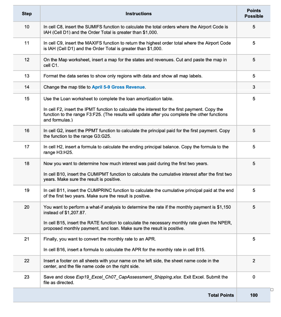
Step Instructions Points Possible 10 5 In cell C8, insert the SUMIFS function to calculate the total orders where the Airport Code is IAH (Cell D1) and the Order Total is greater than $1,000. 11 5 In cell C9, insert the MAXIFS function to return the highest order total where the Airport Code is IAH (Cell D1) and the Order Total is greater than $1,000. 12 On the Map worksheet, insert a map for the states and revenues. Cut and paste the map in cell C1. 5 13 Format the data series to show only regions with data and show all map labels. 5 14 Change the map title to April 5-9 Gross Revenue. 3 15 Use the Loan worksheet to complete the loan amortization table. 5 In cell F2, insert the IPMT function to calculate the interest for the first payment. Copy the function to the range F3:F25. (The results will update after you complete the other functions and formulas.) 16 5 In cell G2, insert the PPMT function to calculate the principal paid for the first payment. Copy the function to the range G3:G25. 17 5 In cell H2, insert a formula to calculate the ending principal balance. Copy the formula to the range H3:H25. 18 Now you want to determine how much interest was paid during the first two years. 5 In cell B10, insert the CUMIPMT function to calculate the cumulative interest after the first two years. Make sure the result is positive. 19 5 In cell B11, insert the CUMPRINC function to calculate the cumulative principal paid at the end of the first two years. Make sure the result is positive. 20 5 You want to perform a what-if analysis to determine the rate if the monthly payment is $1,150 instead of $1,207.87. In cell B15, insert the RATE function to calculate the necessary monthly rate given the NPER, proposed monthly payment, and loan. Make sure the result is positive. 21 Finally, you want to convert the monthly rate to an APR. 5 In cell B16, insert a formula to calculate the APR for the monthly rate in cell B15. 22 2 Insert a footer on all sheets with your name on the left side, the sheet name code in the center, and the file name code on the right side. 23 0 Save and close Exp19_Excel_Ch07_CapAssessment_Shipping.xlsx. Exit Excel. Submit the file as directed Total Points 100 Step Instructions Points Possible 10 5 In cell C8, insert the SUMIFS function to calculate the total orders where the Airport Code is IAH (Cell D1) and the Order Total is greater than $1,000. 11 5 In cell C9, insert the MAXIFS function to return the highest order total where the Airport Code is IAH (Cell D1) and the Order Total is greater than $1,000. 12 On the Map worksheet, insert a map for the states and revenues. Cut and paste the map in cell C1. 5 13 Format the data series to show only regions with data and show all map labels. 5 14 Change the map title to April 5-9 Gross Revenue. 3 15 Use the Loan worksheet to complete the loan amortization table. 5 In cell F2, insert the IPMT function to calculate the interest for the first payment. Copy the function to the range F3:F25. (The results will update after you complete the other functions and formulas.) 16 5 In cell G2, insert the PPMT function to calculate the principal paid for the first payment. Copy the function to the range G3:G25. 17 5 In cell H2, insert a formula to calculate the ending principal balance. Copy the formula to the range H3:H25. 18 Now you want to determine how much interest was paid during the first two years. 5 In cell B10, insert the CUMIPMT function to calculate the cumulative interest after the first two years. Make sure the result is positive. 19 5 In cell B11, insert the CUMPRINC function to calculate the cumulative principal paid at the end of the first two years. Make sure the result is positive. 20 5 You want to perform a what-if analysis to determine the rate if the monthly payment is $1,150 instead of $1,207.87. In cell B15, insert the RATE function to calculate the necessary monthly rate given the NPER, proposed monthly payment, and loan. Make sure the result is positive. 21 Finally, you want to convert the monthly rate to an APR. 5 In cell B16, insert a formula to calculate the APR for the monthly rate in cell B15. 22 2 Insert a footer on all sheets with your name on the left side, the sheet name code in the center, and the file name code on the right side. 23 0 Save and close Exp19_Excel_Ch07_CapAssessment_Shipping.xlsx. Exit Excel. Submit the file as directed Total Points 100