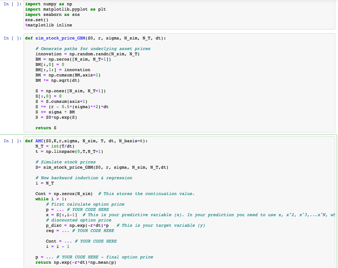
I need help on lines that say # YOUR CODE HERE. (only four segments of code) Thank you!

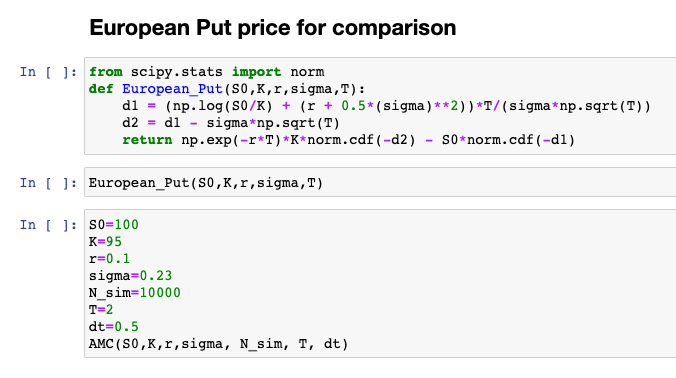
The European Put price is an example usage to try out the function.

original code for copy:

import numpy as np import matplotlib.pyplot as plt import seaborn as sns sns.set() %matplotlib inline

def sim_stock_price_GBM(S0, r, sigma, N_sim, N_T, dt): # Generate paths for underlying asset prices innovation = np.random.randn(N_sim, N_T) BM = np.zeros([N_sim, N_T+1]) BM[:,0] = 0 BM[:,1:] = innovation BM = np.cumsum(BM,axis=1) BM *= np.sqrt(dt)

S = np.ones([N_sim, N_T+1]) S[:,0] = 0 S = S.cumsum(axis=1) S *= (r - 0.5*(sigma)**2)*dt S += sigma * BM S = S0*np.exp(S) return S

def AMC(S0,K,r,sigma, N_sim, T, dt, N_basis=6): N_T = int(T/dt) t = np.linspace(0,T,N_T+1)

# Simulate stock prices S= sim_stock_price_GBM(S0, r, sigma, N_sim, N_T,dt) # Now backward induction & regression i = N_T Cont = np.zeros(N_sim) # This stores the continuation value. while i > 1: # First calculate option price p = ... # YOUR CODE HERE x = S[:,i-1] # This is your predictive variable (x). In your prediction you need to use x, x^2, x^3,...x^N, where N = # of basis # discounted option price p_disc = np.exp(-r*dt)*p # This is your target variable (y) reg = ... # YOUR CODE HERE Cont = ... # YOUR CODE HERE i = i - 1 p = ... # YOUR CODE HERE - final option price return np.exp(-r*dt)*np.mean(p)

from scipy.stats import norm def European_Put(S0,K,r,sigma,T): d1 = (np.log(S0/K) + (r + 0.5*(sigma)**2))*T/(sigma*np.sqrt(T)) d2 = d1 - sigma*np.sqrt(T) return np.exp(-r*T)*K*norm.cdf(-d2) - S0*norm.cdf(-d1)

European_Put(S0,K,r,sigma,T)

S0=100 K=95 r=0.1 sigma=0.23 N_sim=10000 T=2 dt=0.5 AMC(S0,K,r,sigma, N_sim, T, dt)

Thank you!

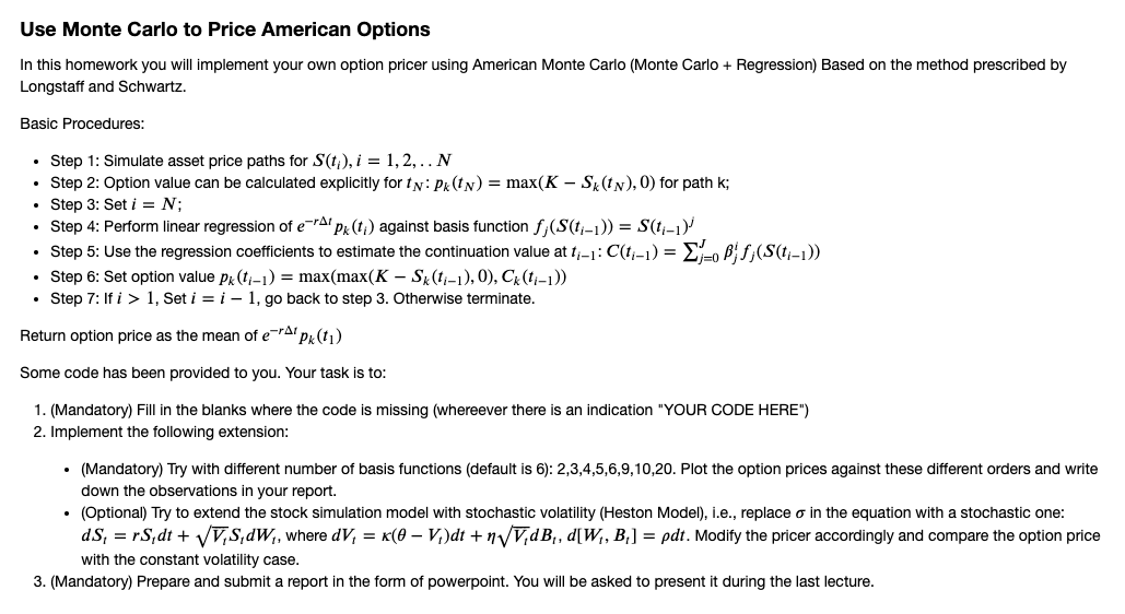
Use Monte Carlo to Price American Options In this homework you will implement your own option pricer using American Monte Carlo (Monte Carlo + Regression) Based on the method prescribed by Longstaff and Schwartz. Basic Procedures: Step 1: Simulate asset price paths for S(ti), i = 1, 2, ..N Step 2: Option value can be calculated explicitly for ty: P (t) = max(K - Sk(tn), O) for path k; Step 3: Set i = N; Step 4: Perform linear regression of e-Alpx(ti) against basis function f;(S(t-1)) = S(t-1) Step 5: Use the regression coefficients to estimate the continuation value at t;1: C(t:-1) = E Bf(S(t1-1)) Step 6: Set option value pr(t-1) = max(max(K - Sk(t-1), 0), C (t-1)) Step 7: If i > 1, Set i =i - 1, go back to step 3. Otherwise terminate. Return option price as the mean of e-px(t1) Some code has been provided to you. Your task is to: 1. (Mandatory) Fill in the blanks where the code is missing (whereever there is an indication "YOUR CODE HERE") 2. Implement the following extension: . (Mandatory) Try with different number of basis functions (default is 6): 2,3,4,5,6,9,10,20. Plot the option prices against these different orders and write down the observations in your report. (Optional) Try to extend the stock simulation model with stochastic volatility (Heston Model), i.e., replace o in the equation with a stochastic one: dS, = rS dt+ VV,S,DW,, where dV, = x(0 - 1)dt + VV,dB,, d[W, B,] = pdt. Modify the pricer accordingly and compare the option price with the constant volatility case. 3. (Mandatory) Prepare and submit a report in the form of powerpoint. You will be asked to present it during the last lecture. In ( ): import numpy as np import matplotlib.pyplot as plt import seaborn as sns sns.set() &matplotlib inline In [ ]: def sim_stock_price_GBM (S0, r, sigma, N_sim, N_T, dt): # Generate paths for underlying asset prices innovation = np.random.randn(N_sim, N_T) BM = np.zeros( [N_sim, N_T+1]) BM[:,0) = 0 BM[:,1:] = innovation BM = np.cumsum (BM, axis=1) BM *= np. sqrt(dt) S = np.ones ( [N_sim, N_T+1]) S[:,0) = 0 S = S.cumsum (axis=1) S *= (r - 0.5*(sigma)**2) *dt S += sigma * BM S = S0*np.exp(S) returns In [ ]: def AMC(S0,K,r, sigma, N_sim, T, dt, N_basis=6): N_T = int(T/dt) t = np.linspace(0,T,N_T+1) # Simulate stock prices S= sim_stock_price_GBM(S0, r, sigma, N_sim, N_T, dt) # Now backward induction & regression i = NUT Cont np.zeros(N_sim) # This stores the continuation value. while i > 1: First calculate option price p= ... # YOUR CODE HERE x = S[:,i-1] # This is your predictive variable (x). In your prediction you need to use x, x^2, x^3,...xN, wh #discounted option price p_disc = np.exp(-r*dt) *p # This is your target variable (y) reg -... # YOUR CODE HERE Cont = ... # YOUR CODE HERE i = i - 1 p = ... # YOUR CODE HERE - final option price return np.exp(-r*dt)*np.mean(p) European Put price for comparison In [ ]: from scipy.stats import norm def European_Put(S0,K,r,sigma, T): d1 = (np.log(SO/K) + (r + 0.5*(sigma)**2)) *T/(sigma*np.sqrt(T)) d2 = di sigma*np.sqrt(T) return np.exp(-r*T)*K*norm.cdf(-d2) SO*norm.cdf(-d1) In [ ]: European_Put (S0,K,r, sigma, T) In ( ): S0=100 K=95 r=0.1 sigma=0.23 N_sim=10000 T=2 dt=0.5 AMC (S0,K,r, sigma, N_sim, T, dt) Use Monte Carlo to Price American Options In this homework you will implement your own option pricer using American Monte Carlo (Monte Carlo + Regression) Based on the method prescribed by Longstaff and Schwartz. Basic Procedures: Step 1: Simulate asset price paths for S(ti), i = 1, 2, ..N Step 2: Option value can be calculated explicitly for ty: P (t) = max(K - Sk(tn), O) for path k; Step 3: Set i = N; Step 4: Perform linear regression of e-Alpx(ti) against basis function f;(S(t-1)) = S(t-1) Step 5: Use the regression coefficients to estimate the continuation value at t;1: C(t:-1) = E Bf(S(t1-1)) Step 6: Set option value pr(t-1) = max(max(K - Sk(t-1), 0), C (t-1)) Step 7: If i > 1, Set i =i - 1, go back to step 3. Otherwise terminate. Return option price as the mean of e-px(t1) Some code has been provided to you. Your task is to: 1. (Mandatory) Fill in the blanks where the code is missing (whereever there is an indication "YOUR CODE HERE") 2. Implement the following extension: . (Mandatory) Try with different number of basis functions (default is 6): 2,3,4,5,6,9,10,20. Plot the option prices against these different orders and write down the observations in your report. (Optional) Try to extend the stock simulation model with stochastic volatility (Heston Model), i.e., replace o in the equation with a stochastic one: dS, = rS dt+ VV,S,DW,, where dV, = x(0 - 1)dt + VV,dB,, d[W, B,] = pdt. Modify the pricer accordingly and compare the option price with the constant volatility case. 3. (Mandatory) Prepare and submit a report in the form of powerpoint. You will be asked to present it during the last lecture. In ( ): import numpy as np import matplotlib.pyplot as plt import seaborn as sns sns.set() &matplotlib inline In [ ]: def sim_stock_price_GBM (S0, r, sigma, N_sim, N_T, dt): # Generate paths for underlying asset prices innovation = np.random.randn(N_sim, N_T) BM = np.zeros( [N_sim, N_T+1]) BM[:,0) = 0 BM[:,1:] = innovation BM = np.cumsum (BM, axis=1) BM *= np. sqrt(dt) S = np.ones ( [N_sim, N_T+1]) S[:,0) = 0 S = S.cumsum (axis=1) S *= (r - 0.5*(sigma)**2) *dt S += sigma * BM S = S0*np.exp(S) returns In [ ]: def AMC(S0,K,r, sigma, N_sim, T, dt, N_basis=6): N_T = int(T/dt) t = np.linspace(0,T,N_T+1) # Simulate stock prices S= sim_stock_price_GBM(S0, r, sigma, N_sim, N_T, dt) # Now backward induction & regression i = NUT Cont np.zeros(N_sim) # This stores the continuation value. while i > 1: First calculate option price p= ... # YOUR CODE HERE x = S[:,i-1] # This is your predictive variable (x). In your prediction you need to use x, x^2, x^3,...xN, wh #discounted option price p_disc = np.exp(-r*dt) *p # This is your target variable (y) reg -... # YOUR CODE HERE Cont = ... # YOUR CODE HERE i = i - 1 p = ... # YOUR CODE HERE - final option price return np.exp(-r*dt)*np.mean(p) European Put price for comparison In [ ]: from scipy.stats import norm def European_Put(S0,K,r,sigma, T): d1 = (np.log(SO/K) + (r + 0.5*(sigma)**2)) *T/(sigma*np.sqrt(T)) d2 = di sigma*np.sqrt(T) return np.exp(-r*T)*K*norm.cdf(-d2) SO*norm.cdf(-d1) In [ ]: European_Put (S0,K,r, sigma, T) In ( ): S0=100 K=95 r=0.1 sigma=0.23 N_sim=10000 T=2 dt=0.5 AMC (S0,K,r, sigma, N_sim, T, dt)