I need it as soon as possible please

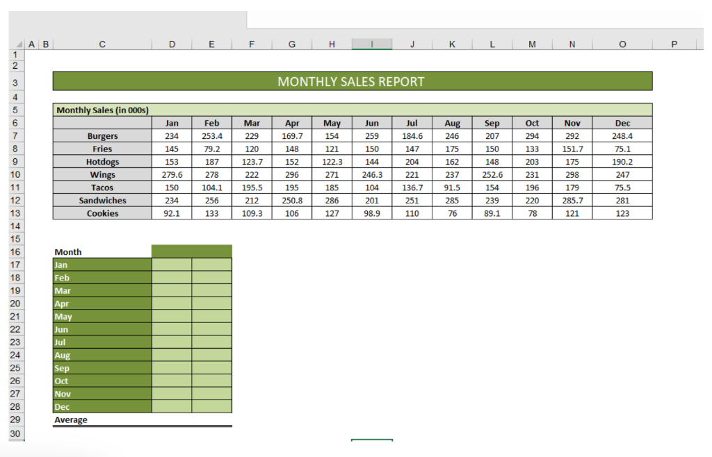
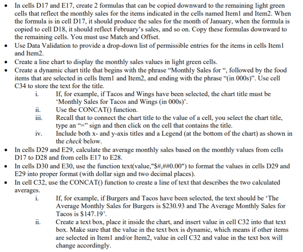
D E F G H K. L M N P 1 2 3 MONTHLY SALES REPORT 4 5 Monthly Sales (in 000s) Mar Nov 6 7 Apr 169.7 Jun 259 May 154 121 Aug 246 J Oct 294 229 Sep 207 150 150 175 133 8 9 9 10 148 152 296 144 Burgers Fries Hotdogs Wings Tacos Sandwiches Cookies Jan 234 145 153 279.6 150 234 92.1 Feb 253.4 79.2 187 278 104.1 256 133 292 151.7 175 298 148 203 Jul 184.6 147 204 221 136.7 251 Dec 248.4 75.1 190.2 247 75.5 | 120 123.7 222 195.5 212 109.3 122.3 271 185 IT 246.3 104 162 237 91.5 285 DU 252.6 154 231 196 195 HHHH 11 12 179 II 286 220 250.8 106 201 98.9 239 89.1 285.7 121 281 123 127 110 76 78 13 14 15 16 17 18 19 20 21 22 23 24 25 26 27 28 Month Jan Feb Mar Apr May Jun Jul Aug Sep Oct Nov Dec Average 29 30 In cells D17 and E17, create 2 formulas that can be copied downward to the remaining light green cells that reflect the monthly sales for the items indicated in the cells named Iteml and Item2. When the formula is in cell D17, it should produce the sales for the month of January, when the formula is copied to cell D18, it should reflect February's sales, and so on. Copy these formulas downward to the remaining cells. You must use Match and Offset. Use Data Validation to provide a drop-down list of permissible entries for the items in cells Iteml and Item2. Create a line chart to display the monthly sales values in light green cells. Create a dynamic chart title that begins with the phrase Monthly Sales for , followed the food items that are selected in cells Iteml and Item2, and ending with the phrase (in 000s). Use cell C34 to store the text for the title. i. If, for example, if Tacos and Wings have been selected, the chart title must be Monthly Sales for Tacos and Wings (in 000s)'. ii. Use the CONCAT() function. iii. Recall that to connect the chart title to the value of a cell, you select the chart title, type an = sign and then click on the cell that contains the title. iv. Include both x- and y-axis titles and a Legend (at the bottom of the chart) as shown in the check below. In cells D29 and E29, calculate the average monthly sales based on the monthly values from cells D17 to D28 and from cells E17 to E28. In cells D30 and E30, use the function text(value,"$#,##0.00") to format the values in cells D29 and E29 into proper format (with dollar sign and two decimal places). In cell C32, use the CONCAT() function to create a line of text that describes the two calculated averages. If, for example, if Burgers and Tacos have been selected, the text should be The Average Monthly Sales for Burgers is $230.93 and The Average Monthly Sales for Tacos is $147.19'. ii. Create a text box, place it inside the chart, and insert value in cell C32 into that text box. Make sure that the value in the text box is dynamic, which means if other items are selected in Iteml and/or Item2, value in cell C32 and value in the text box will change accordingly. i. D E F G H K. L M N P 1 2 3 MONTHLY SALES REPORT 4 5 Monthly Sales (in 000s) Mar Nov 6 7 Apr 169.7 Jun 259 May 154 121 Aug 246 J Oct 294 229 Sep 207 150 150 175 133 8 9 9 10 148 152 296 144 Burgers Fries Hotdogs Wings Tacos Sandwiches Cookies Jan 234 145 153 279.6 150 234 92.1 Feb 253.4 79.2 187 278 104.1 256 133 292 151.7 175 298 148 203 Jul 184.6 147 204 221 136.7 251 Dec 248.4 75.1 190.2 247 75.5 | 120 123.7 222 195.5 212 109.3 122.3 271 185 IT 246.3 104 162 237 91.5 285 DU 252.6 154 231 196 195 HHHH 11 12 179 II 286 220 250.8 106 201 98.9 239 89.1 285.7 121 281 123 127 110 76 78 13 14 15 16 17 18 19 20 21 22 23 24 25 26 27 28 Month Jan Feb Mar Apr May Jun Jul Aug Sep Oct Nov Dec Average 29 30 In cells D17 and E17, create 2 formulas that can be copied downward to the remaining light green cells that reflect the monthly sales for the items indicated in the cells named Iteml and Item2. When the formula is in cell D17, it should produce the sales for the month of January, when the formula is copied to cell D18, it should reflect February's sales, and so on. Copy these formulas downward to the remaining cells. You must use Match and Offset. Use Data Validation to provide a drop-down list of permissible entries for the items in cells Iteml and Item2. Create a line chart to display the monthly sales values in light green cells. Create a dynamic chart title that begins with the phrase Monthly Sales for , followed the food items that are selected in cells Iteml and Item2, and ending with the phrase (in 000s). Use cell C34 to store the text for the title. i. If, for example, if Tacos and Wings have been selected, the chart title must be Monthly Sales for Tacos and Wings (in 000s)'. ii. Use the CONCAT() function. iii. Recall that to connect the chart title to the value of a cell, you select the chart title, type an = sign and then click on the cell that contains the title. iv. Include both x- and y-axis titles and a Legend (at the bottom of the chart) as shown in the check below. In cells D29 and E29, calculate the average monthly sales based on the monthly values from cells D17 to D28 and from cells E17 to E28. In cells D30 and E30, use the function text(value,"$#,##0.00") to format the values in cells D29 and E29 into proper format (with dollar sign and two decimal places). In cell C32, use the CONCAT() function to create a line of text that describes the two calculated averages. If, for example, if Burgers and Tacos have been selected, the text should be The Average Monthly Sales for Burgers is $230.93 and The Average Monthly Sales for Tacos is $147.19'. ii. Create a text box, place it inside the chart, and insert value in cell C32 into that text box. Make sure that the value in the text box is dynamic, which means if other items are selected in Iteml and/or Item2, value in cell C32 and value in the text box will change accordingly