Question
I was given the following file ScriptFigs.m: % % Script for generating figures and testing stuff. % n = 10; x = 1:n; y =


I was given the following file "ScriptFigs.m":
% % Script for generating figures and testing stuff. %
n = 10;
x = 1:n; y = randn(n,1);
pp = spline (x, y);
%% Plot the results
delta = 0.05; x2 = 1:delta:n;
figure; plot (x2, ppval(pp, x2)); hold on; plot (x, y, 'ro'); hold off;
%% 2D Spline
% create an axis
figure; axis([-10 10 -10 10]);
[X, Y] = getpts();
N = length(X);
ppx = spline (1:N, X); ppy = spline (1:N, Y);
delta = 0.01;
X2 = ppval (1:delta:N, ppx); Y2 = ppval (1:delta:N, ppy);
hold on; plot (X2, Y2); plot (X, Y, 'ro');
and the file "examplelinearsystems":
% % Examples of Linear Systems %
%% Example 1 - 1D interpolation: % Given the value of a function y = a x^3 + b x^2 + c x + d at a few points % recover the coefficients z, b, c and d and hence the value of the % function everyhere
x1 = 0.10; y1 = -3.3;
x2 = 0.20; y2 = 10.0;
x3 = 0.55; y3 = -1.0; x4 = 0.75; y4 = 2.2;
figure; plot ([x1 x2 x3 x4], [y1 y2 y3 y4], 'r*');
% Set up the linear system - one equation for every correspondence A = [x1^3 x1^2 x1 1; ... x2^3 x2^2 x2 1; ... x3^3 x3^2 x3 1; ... x4^3 x4^2 x4 1; ... ];
b = [y1 y2 y3 y4]';
% Solve for the coefficients coeffs = A \ b;
% Plot the function hold on;
x = 0:0.01:1;
y = coeffs(1)*x.^3 + coeffs(2)*x.^2 + coeffs(3)*x + coeffs(4);
plot (x, y);
%% Example 2 - 2D interpolation: % Given the value of a function of 2 variables % z = f(x,y) = a x^2 + b xy + cy^2 + dx + ey + f % recover all of the coefficients and hence the value everywhere
x1 = 1.0; y1 = 1.0; z1 = 0.5; x2 = 2.0; y2 = -1.0; z2 = -2.0; x3 = 3.0; y3 = 5.0; z3 = -14.4282; x4 = -1.0; y4 = 1.0; z4 = 4.5; x5 = -2.0; y5 = 1.5; z5 = 11.3391; x6 = 0.0; y6 = 3.0; z6 = 6.9282;
% Set up the linear system A = [ x1^2 x1*y1 y1^2 x1 y1 1; ... x2^2 x2*y2 y2^2 x2 y2 1; ... x3^2 x3*y3 y3^2 x3 y3 1; ... x4^2 x4*y4 y4^2 x4 y4 1; ... x5^2 x5*y5 y5^2 x5 y5 1; ... x6^2 x6*y6 y6^2 x6 y6 1; ... ];
b = [z1 z2 z3 z4 z5 z6]';
% Solve for the coefficients coeffs = A \ b;
% plot the function
[X, Y] = meshgrid([-5:0.1:5], [-5:0.1:5]);
Z = coeffs(1).*X.^2 + coeffs(2).*X.*Y + coeffs(3).*Y.^2 + coeffs(4)*X + coeffs(5)*Y + coeffs(6);
figure; surf (X, Y, Z); hold on;
plot3 ([x1 x2 x3 x4 x5 x6], [y1 y2 y3 y4 y5 y6], [z1 z2 z3 z4 z5 z6], 'r*');
%% Stretchy rope example
N = 50;
m = 0.1; M = 2.5; g = 9.8; k = 5.0;
% Index of the node with the weight idx = 30;
A = zeros(N); b = zeros(N,1);
% Set up the linear system.
for i = 2:(N-1) A(i,i-1) = k; A(i,i) = -2*k; A(i,i+1) = k; b(i) = m * g; end
% Fixed end points A(1,1) = 1; b(1) = 0;
A(N,N) = 1; b(N) = 0;
% Special equation for the node with the weight
b(idx) = (m + M) * g;
% Solve for the displacement y = A \ b;
% Plot figure; plot (1:N, y, 'r.', 'MarkerSize', 5); hold on; plot (1:N, y, 'b'); hold off;
%% Look at the structure of the stretchy rope system (tridiagonal)
figure; spy(A);
% Allocate a sparse matrix, N x N A2 = spalloc(N,N, 3*N);
% Set up the linear system.
for i = 2:(N-1) A2(i,i-1) = k; A2(i,i) = -2*k; A2(i,i+1) = k; end
% Fixed end points A2(1,1) = 1; A2(N,N) = 1;
figure; spy(A2);
nnz(A2);
% Matlab will recognize that A2 is sparse and tridiagonal and invoke an % efficient algorithm for this case. You don't have to do anything special. y2 = A2 \ b;
%% Poisson Equation example
% Define an N x N grid N = 50;
A = eye(N*N, N*N);
b = zeros(N, N);
% Fill in equations for the central elements according to the Poisson % equation
for i = 2:N-1 for j = 2:N-1 idx = sub2ind([N N], i, j); A(idx, idx) = -4; A(idx, idx+1) = 1; A(idx, idx-1) = 1; A(idx, idx-N) = 1; A(idx, idx+N) = 1; end end
% Boundary conditions % Set the temperature along side1
b(:,1) = 1:N; b(1,:) = 1:N; b(N,:) = N:-1:1;
% Solve the PDE with boundary conditions temp = A \ b(:);
% Plot the answer figure; mesh(reshape(temp, N, N));
%% Look at the structure of the Poisson system
spy(A);
A2 = sparse(A);
whos A A2;
tic; temp2 = A2 \ b(:); toc;
tic; temp = A \ b(:); toc;
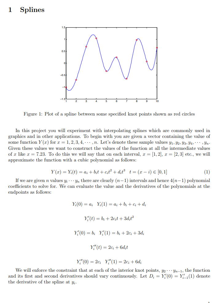
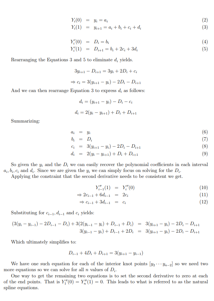
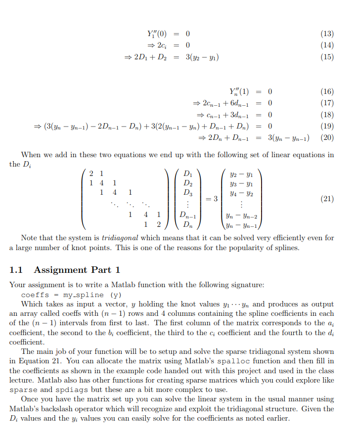
1 Splines 1.5 0.5 -0.5 Figure 1: Plot of a spline between some specified knot points shown as red circles In this project you will experiment with interpolating s graphics and in other applications. To begin with you are given a vector containing the value of some function Y (x) for x-1, 2, 3, 4, . . . , n. Let's denote these sample values y, , , 3a,' . . , yn Given these values we want to construct the values of the function at all the intermediate values of! like ! = 7.23. To do this we will say that on each interval, x = [1,2], x = [2,3] etc., we will approximate the function with a cubic polynomial as follows plines which are commonly used in If we are given n values yi Yn there are clearly (n-1) intervals and hence 4(n-1) polynomial coefficients to solve for. We can evaluate the value and the derivatives of the polynomials at the endpoints as follows "(t) = 2c; + 6dit We will enforce the constraint that at each of the interior knot points, y2 .yn-1, the function and its first and second derivatives should vary continuously. Let Di = Y,(0) = 1(1) denote the derivative of the spline at y Rearranging the Equations 3 and 5 to eliminate d, yields. And we can then rearrange Equation 3 to express di as follows: Summarizing: ai yi d; 2(Vi-Vi+1) + Di + Di+1 = So given the yi and the Di we can easily recover the polynomial coefficients in each interval a,, b,c, and d,. Since we are given the y we can simply focus on solving for the D Applying the constraint that the second derivative needs to be consistent we get (10) (12) Substituting for ci-1,d,-1 and c yields Which ultimately simplifies to We have one such equation for each of the interior knot points y2yn-2] so we need two more equations so we can solve for all n values of D One way to get the remaining two equations is to set the second derivative to zero at each of the end points. That is Y"(0) = Y,"(1) = 0, This leads to what is referred to as the natural spline equations (13) (14) (15) (16) (17) (18) (19) 2D, + Dn-1 = 3(Yn-Yn-1) (20) When we add in these two equations we end up with the following set of linear equations in the D (21) 1 41 Note that the system is tridiagonal which means that it can be solved very efficiently even for a large number of knot points. This is one of the reasons for the popularity of splines. 1.1 Assignment Part 1 Your assignment is to write a Matlab function with the following signature coeffs my-spline (y) = Which takes as input a vector, y holding the knot values yn and produces as output an array called coeffs with (n -1) rows and 4 columns containing the spline coefficients in each of the (n-1) intervals from first to last. The first column of the matrix corresponds to the a, coefficient, the second to the bi coefficient, the third to the ci coefficient and the fourth to the d, coefficient The main job of your function will be to setup and solve the sparse tridiagonal system shown in Equation 21. You can allocate the matrix using Matlab's spalloc function and then fill in the coefficients as shown in the example code handed out with this project and used in the class lecture. Matlab also has other functions for creating sparse matrices which you could explore like sparse and spdiags but these are a bit more complex to use Once you have the matrix set up you can solve the linear system in the usual manner using e and exploit the tridiagonal structure. Given the Matlab's backslash operator which will reco Di values and the yi values you can easily solve for the coefficients as noted earlier gniz 1 Splines 1.5 0.5 -0.5 Figure 1: Plot of a spline between some specified knot points shown as red circles In this project you will experiment with interpolating s graphics and in other applications. To begin with you are given a vector containing the value of some function Y (x) for x-1, 2, 3, 4, . . . , n. Let's denote these sample values y, , , 3a,' . . , yn Given these values we want to construct the values of the function at all the intermediate values of! like ! = 7.23. To do this we will say that on each interval, x = [1,2], x = [2,3] etc., we will approximate the function with a cubic polynomial as follows plines which are commonly used in If we are given n values yi Yn there are clearly (n-1) intervals and hence 4(n-1) polynomial coefficients to solve for. We can evaluate the value and the derivatives of the polynomials at the endpoints as follows "(t) = 2c; + 6dit We will enforce the constraint that at each of the interior knot points, y2 .yn-1, the function and its first and second derivatives should vary continuously. Let Di = Y,(0) = 1(1) denote the derivative of the spline at y Rearranging the Equations 3 and 5 to eliminate d, yields. And we can then rearrange Equation 3 to express di as follows: Summarizing: ai yi d; 2(Vi-Vi+1) + Di + Di+1 = So given the yi and the Di we can easily recover the polynomial coefficients in each interval a,, b,c, and d,. Since we are given the y we can simply focus on solving for the D Applying the constraint that the second derivative needs to be consistent we get (10) (12) Substituting for ci-1,d,-1 and c yields Which ultimately simplifies to We have one such equation for each of the interior knot points y2yn-2] so we need two more equations so we can solve for all n values of D One way to get the remaining two equations is to set the second derivative to zero at each of the end points. That is Y"(0) = Y,"(1) = 0, This leads to what is referred to as the natural spline equations (13) (14) (15) (16) (17) (18) (19) 2D, + Dn-1 = 3(Yn-Yn-1) (20) When we add in these two equations we end up with the following set of linear equations in the D (21) 1 41 Note that the system is tridiagonal which means that it can be solved very efficiently even for a large number of knot points. This is one of the reasons for the popularity of splines. 1.1 Assignment Part 1 Your assignment is to write a Matlab function with the following signature coeffs my-spline (y) = Which takes as input a vector, y holding the knot values yn and produces as output an array called coeffs with (n -1) rows and 4 columns containing the spline coefficients in each of the (n-1) intervals from first to last. The first column of the matrix corresponds to the a, coefficient, the second to the bi coefficient, the third to the ci coefficient and the fourth to the d, coefficient The main job of your function will be to setup and solve the sparse tridiagonal system shown in Equation 21. You can allocate the matrix using Matlab's spalloc function and then fill in the coefficients as shown in the example code handed out with this project and used in the class lecture. Matlab also has other functions for creating sparse matrices which you could explore like sparse and spdiags but these are a bit more complex to use Once you have the matrix set up you can solve the linear system in the usual manner using e and exploit the tridiagonal structure. Given the Matlab's backslash operator which will reco Di values and the yi values you can easily solve for the coefficients as noted earlier gnizStep by Step Solution
There are 3 Steps involved in it
Step: 1

Get Instant Access to Expert-Tailored Solutions
See step-by-step solutions with expert insights and AI powered tools for academic success
Step: 2

Step: 3

Ace Your Homework with AI
Get the answers you need in no time with our AI-driven, step-by-step assistance
Get Started


