I would like to summarize this section, with an example for clarification, please

Discrete Units The EOQ, as given by Equation 4.4, will likely result in a nonintegral number of units. However, it can be shown mathematically (and is obvious from the form of the total cost curve of Figure 4.2) that the best integer value of Q has to be one of the two integers surrounding the best (noninteger) solution given by Equation 4.4. For simplicity, we recommend simply rounding the result of Equation 4.4, that is, the EOQ, to the nearest integer.*

Certain commodities are sold in pack sizes containing more than one unit; for example, many firms sell in pallet-sized loads only, say 48 units (e.g., cases). Therefore, it makes sense to restrict a replenishment quantity to integer multiples of 48 units. In fact, if a new unit, corresponding to 48 of the old unit, is defined, then, we are back to the basic situation of requiring an integer number of (the new) units in a replenishment quantity.

There is another possible restriction on the replenishment quantity that is very similar to that of discrete units. This is the situation where the replenishment must cover an integral number of periods of demand. Again, we simply find the optimal continuous Q expressed as a time supply (see Equation 4.7) and round to the nearest integer value of the time supply.

E.q 4.4

E.q 4.6

i need just Discrete Units

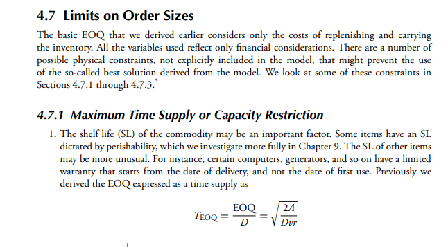
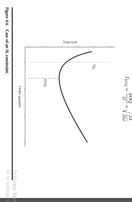
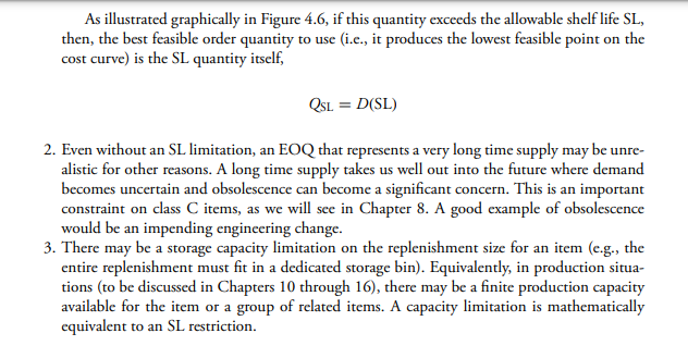
Economic Order Quantity =ur2AD TEOQ=D12EOQ=rDu288A 4.7 Limits on Order Sizes The basic EOQ that we derived earlier considers only the costs of replenishing and carrying the inventory. All the variables used reflect only financial considerations. There are a number of possible physical constraints, not explicitly included in the model, that might prevent the use of the so-called best solution derived from the model. We look at some of these constraints in Sections 4.7.1 through 4.7.3." 4.7.1 Maximum Time Supply or Capacity Restriction 1. The shelf life (SL) of the commodity may be an important factor. Some items have an SL dictated by perishability, which we investigate more fully in Chapter 9 . The SL of other items may be more unusual. For instance, certain computers, generators, and so on have a limited warranty that starts from the date of delivery, and not the date of first use. Previously we derived the EOQ expressed as a time supply as TEOQ=DEOQ=Dvr2A TEOQ=DEOQ=Dvr2A Figure 4.6 Case of an SL constraint. As illustrated graphically in Figure 4.6, if this quantity exceeds the allowable shelf life SL, then, the best feasible order quantity to use (i.e., it produces the lowest feasible point on the cost curve) is the SL quantity itself, QSL=D(SL) 2. Even without an SL limitation, an EOQ that represents a very long time supply may be unrealistic for other reasons. A long time supply takes us well out into the future where demand becomes uncertain and obsolescence can become a significant concern. This is an important constraint on class C items, as we will see in Chapter 8 . A good example of obsolescence would be an impending engineering change. 3. There may be a storage capacity limitation on the replenishment size for an item (e.g., the entire replenishment must fit in a dedicated storage bin). Equivalently, in production situations (to be discussed in Chapters 10 through 16), there may be a finite production capacity available for the item or a group of related items. A capacity limitation is mathematically equivalent to an SL restriction. Economic Order Quantity =ur2AD TEOQ=D12EOQ=rDu288A 4.7 Limits on Order Sizes The basic EOQ that we derived earlier considers only the costs of replenishing and carrying the inventory. All the variables used reflect only financial considerations. There are a number of possible physical constraints, not explicitly included in the model, that might prevent the use of the so-called best solution derived from the model. We look at some of these constraints in Sections 4.7.1 through 4.7.3." 4.7.1 Maximum Time Supply or Capacity Restriction 1. The shelf life (SL) of the commodity may be an important factor. Some items have an SL dictated by perishability, which we investigate more fully in Chapter 9 . The SL of other items may be more unusual. For instance, certain computers, generators, and so on have a limited warranty that starts from the date of delivery, and not the date of first use. Previously we derived the EOQ expressed as a time supply as TEOQ=DEOQ=Dvr2A TEOQ=DEOQ=Dvr2A Figure 4.6 Case of an SL constraint. As illustrated graphically in Figure 4.6, if this quantity exceeds the allowable shelf life SL, then, the best feasible order quantity to use (i.e., it produces the lowest feasible point on the cost curve) is the SL quantity itself, QSL=D(SL) 2. Even without an SL limitation, an EOQ that represents a very long time supply may be unrealistic for other reasons. A long time supply takes us well out into the future where demand becomes uncertain and obsolescence can become a significant concern. This is an important constraint on class C items, as we will see in Chapter 8 . A good example of obsolescence would be an impending engineering change. 3. There may be a storage capacity limitation on the replenishment size for an item (e.g., the entire replenishment must fit in a dedicated storage bin). Equivalently, in production situations (to be discussed in Chapters 10 through 16), there may be a finite production capacity available for the item or a group of related items. A capacity limitation is mathematically equivalent to an SL restriction